How to use Excel XLOOKUP Function

XLOOKUP finds the lookup value in a vertical or horizontal array and supports exact match, wildcards, and binary search.

Table of contents:

• What is XLOOKUP
• How can I get XLOOKUP
• How to use XLOOKUP Function
  • Syntax, Arguments
  • Basic usage, exact match (required arguments only)
  • “if not found” argument (4th argument)
  • Match mode or type (5th argument)
  • Search mode (6th argument)
• XLOOKUP Function Examples
  • Lookup right to left
  • Combine XLOOKUP with the MIN or MAX functions
  • Replace INDEX and MATCH functions
  • Approximate Match mode: Find the next smaller item (closest value)
  • Approximate Match mode: Find the next larger item (closest value)
  • Wildcard character match (* or ?)
  • Last to first search mode
  • First to last search mode
  • Binary search
  • Multiple results
• Why XLOOKUP is better than other lookups (VLOOKUP, HLOOKUP, INDEX, and MATCH)
• XLOOKUP Formulas
• Why XLOOKUP is not working properly

What is XLOOKUP?

XLOOKUP is a game-changer, a powerful and versatile lookup function in Excel. It provides flexible solutions to replace the older lookup functions, like VLOOKUP, HLOOKUP, LOOKUP, and the INDEX+MATCH combination. The function supports horizontal lookups and vertical lookups. Furthermore, it simplifies your formulas.

How can I get XLOOKUP?

XLOOKUP is only available for Microsoft 365 (formerly Office 365) users. In addition, you cannot use the function if you use an older version of Microsoft Excel (2010, 2013, 2016, 2019). That was the official information, but using it with any Excel version is tricky.

If you want to use XLOOKUP with the recent Excel versions, check our add-in, which provides the latest lookup functionality for all Microsoft Excel versions. Alternatively, you can replace the function in the case of the xlfn prefix.

Download the sample workbook and play with it. The Practice Workbook contains all questions and answers using a single formula.

Download the practice file.

Use names for a range to make your learning curve fast and more straightforward.

How to use XLOOKUP Function

This section will explain how the XLOOKUP syntax and arguments work.

Syntax, Arguments

XLOOKUP uses the following syntax:

=XLOOKUP(lookup_value, lookup_array, return_array, [if_not_found], [match_mode], [search_mode])

XLOOKUP is similar to the VLOOKUP function but uses six arguments. Three arguments are required, and another three are optional.

Required arguments:

• The value you are looking for: lookup_value
• The list where we find the lookup value: lookup_array
• The list from which you want the result: return_array

Optional arguments:

• Error handling; what if the value is not found: not_found
• Declare match types: match_mode
• Controls the search action: search_mode

Before we use the XLOOKUP function in Excel, it is worth creating named ranges. The process can take seconds, and we will get an easy-to-understand structure for your data set. To create a named range, select the range you want to name, locate the name box and type a name – finally, press Enter. Once the data set is ready, we can build various lookup formulas.

Note: In this tutorial, we use Microsoft 365.

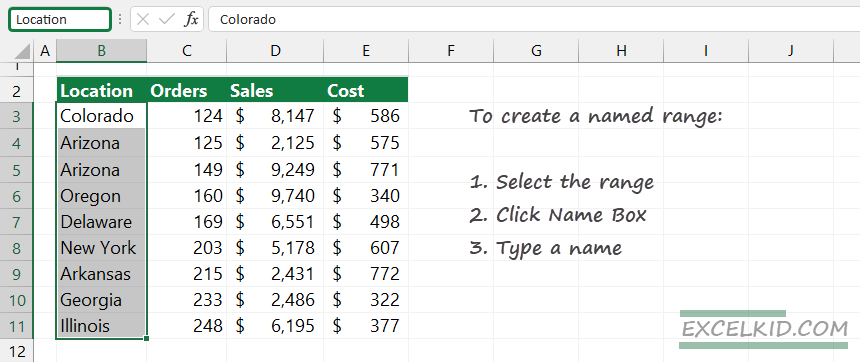
We will use four named ranges:

• Location = B3: B11
• Orders = C3: C11
• Sales = D3: D11
• Cost = E3: E11

XLOOKUP works fine using classic cell references, but structured references provide easy-to-understand formulas.

Basic usage, exact match (required arguments only)

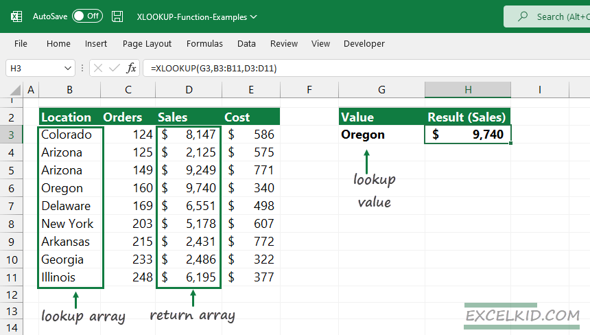
In the example below, we want to find the Sales for New York to return the “Sales” based on an exact match in the list, “Location”.

Good to know that by default, XLOOKUP returns an exact match; no additional argument is necessary.

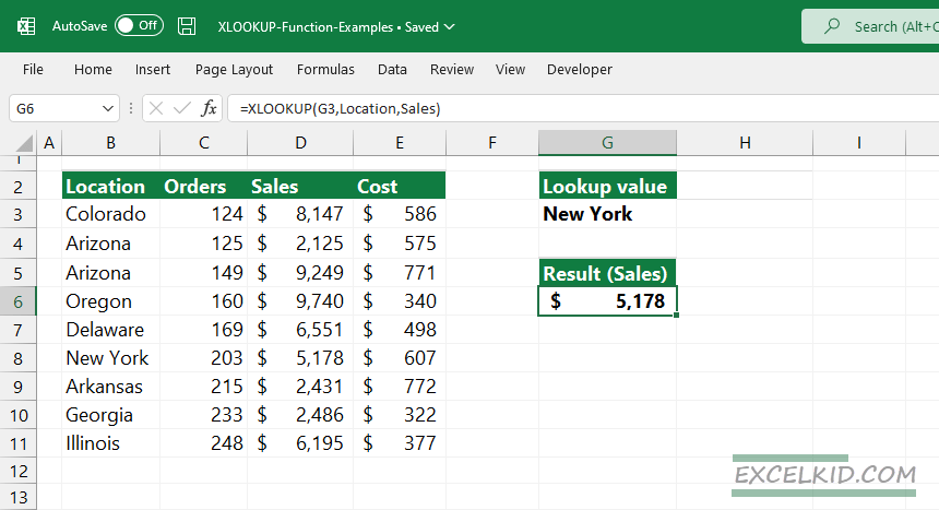
General formula:

=XLOOKUP(what we want to find, lookup list, result list)

=XLOOKUP(G3, Location, Sales)

Explanation: The formula finds the lookup value in the lookup array and returns $5178 if the lookup value is available in column B. For simplicity, we use the above-mentioned named ranges.

XLOOKUP “if not found” argument (4th argument)

XLOOKUP returns the #N/A error when not finding a match in a return array and all other Excel lookup functions get the same error message.

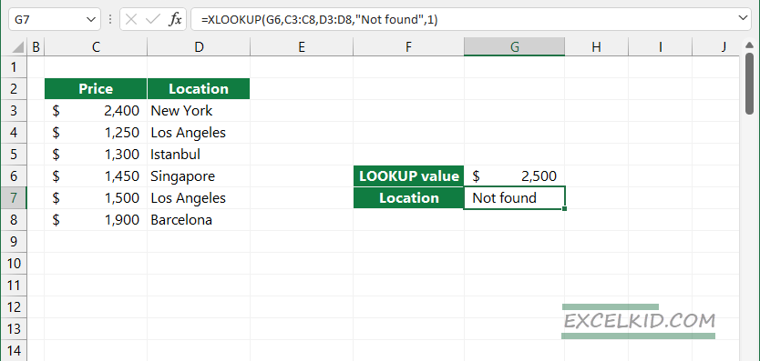
The function uses an optional argument that supports error handling in place without using additional functions. You can choose two practical ways to create a more user-friendly output in case of no match. First, apply double quotes (“”) to build an empty string result.

Furthermore, you can customize the message when the formula does not find a matching value. For example, choose an easy-to-understand string instead of #N/A, like: “not found”, “no result”, or “value not found”.

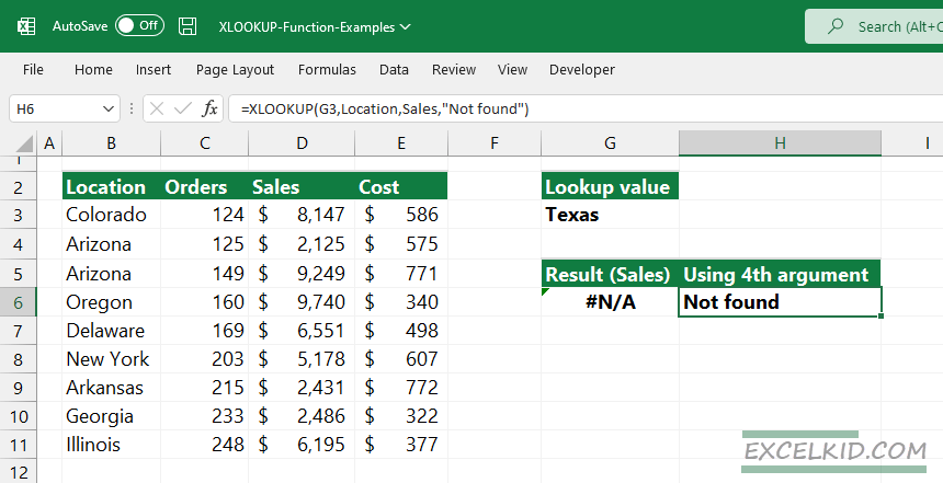
In the example, find the sales where the location is Texas. What if the lookup array does not contain the lookup value? Without using the 4th argument, the result is an #N/A error. Use the optional 4th argument to create a string instead of the #N/A error.

Error handling formula using XLOOKUP:

=XLOOKUP(G3, Location, Sales, “Not found”)

Explanation: The formula returns the “Not found” string if the lookup value (Texas) is unavailable in column B.

Match mode or type (5th argument)

Use the match mode argument as a 5th argument of XLOOKUP to declare in Excel how you want your MATCH to happen. These are the following:

Match type	Action
0 (default)	Exact match (returns #N/A if no match.)
-1	Exact match or the next smaller item (approximate match)
1	Exact match or the next larger item (approximate match)
2	Wildcard match

Search mode (6th argument)

Good to know that XLOOKUP will start matching from the first data value by default. The search_mode optional argument controls the search action and uses the following options:

Search Mode	Action
1 (default)	Search from the first value; the array contains unsorted values.
-1	Search from the last value in an array (reverse search)
2	Binary search: values sorted in ascending order
-2	Binary search: values sorted in descending order

XLOOKUP Function Examples

Lookup right to the left using XLOOKUP

XLOOKUP has native left lookup support. Therefore, you can use it instead of VLOOKUP and CHOOSE-based formulas.

In the example, our data set contains the following columns: Location, Orders, Sales, and Cost. We want to find the location in column B, where the cost = is $498. Therefore, the lookup array is E3:E13 (Cost), and the return array is B3:B13 (Location).

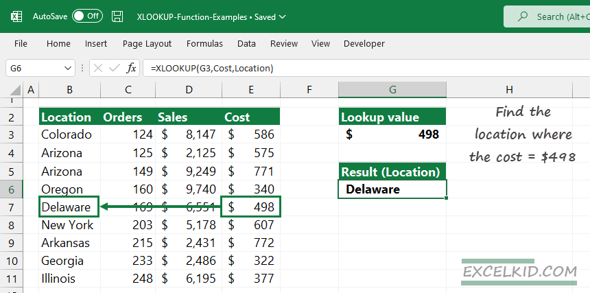
Use the following formula to lookup right to left:

=XLOOKUP(G3, Cost, Location)

If your Excel version does not support XLOOKUP, here is a right-to-left workaround with the VLOOKUP and CHOOSE functions. First, use the CHOOSE function to restructure the lookup table and replace the Sales and Location columns.

=CHOOSE({1,2}, Cost, Location)

VLOOKUP function will perform the usual left-to-right lookup and return with the matching location based on the lookup value.

Formula:

=VLOOKUP(G3,CHOOSE({1,2},Cost,Location), 2, 0)

Combine XLOOKUP with the MIN or MAX functions

You can easily combine XLOOKUP with Excel functions like MIN or MAX. In the example, we will use XLOOKUP with the MIN function to return the minimum sales with the corresponding location.

Formula:

=XLOOKUP(MIN(Sales), Sales, Location)

Use the following arguments:

• lookup value: MIN(Sales)
• lookup array: Sales
• return array: Location

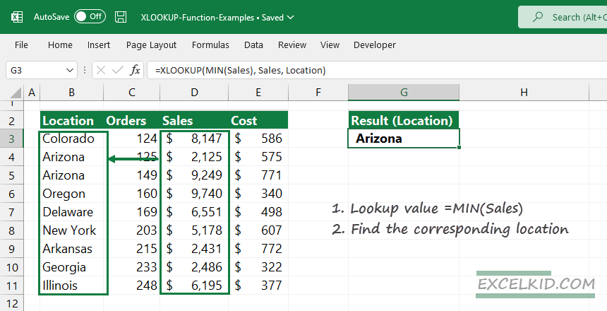
Explanation: The =MIN(Sales) expression returns with the minimum value in the Sales array. Therefore the lookup value is based on the result of the MIN function. Finally, XLOOKUP will use the result as a lookup value.

Replace INDEX and MATCH functions

One of the benefits of using XLOOKUP is that it completely replaces the INDEX and MATCH-based formulas. In the example, we aim to find the ‘Orders’ where the ‘Sales’ = $2486.

Configure the arguments:

• lookup value = 2486
• lookup array = Sales
• return array = Orders

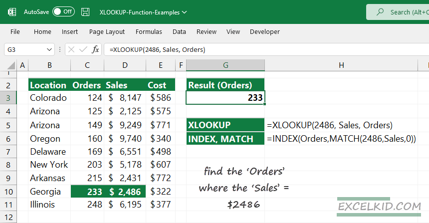
Formula:

=XLOOKUP(2486, Sales, Orders)

The result is Oregon because here, we have 160 orders.

Okay, that was easy! Let us see what will happen if we don’t have XLOOKUP. Now we explain the possible workaround with the INDEX and MATCH combinations.

INDEX and MATCH formula:

=INDEX(Orders, MATCH(2486, Sales, 0))

Evaluate the formula working from the inside out. Next, the MATCH function finds the lookup value (2486) in the Sales column and returns with row number 8. Finally, INDEX will use the row number as a second argument.

You can easily decide which formula is shorter, better, and more flexible.

XLOOKUP Match mode: Find the next smaller item (closest value)

It’s time to take a closer look at the XLOOKUP match types. We used exact match (default value = 0) as a match_mode. The following example will demonstrate the power of an approximate match mode. The fifth argument of the function is a swiss-knife. We will show you why.

With XLOOKUP, you can use the -1 parameter as a match mode argument to find the next smaller item, the closest value.

In the example, our lookup value is $5200 in the sales column, and we try to find the location where the sales are less than or equal to $5200.

Formula:

=XLOOKUP(G3, Sales, Location,,-1)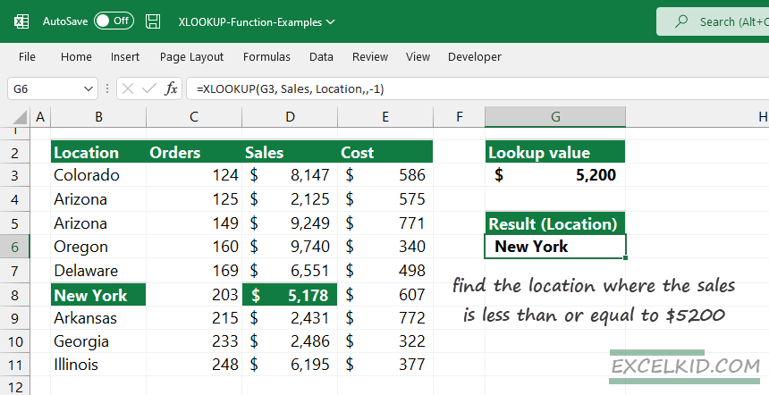

The result is New York.

Explanation: First, the formula tries to search for an exact match. There is no exact match; XLOOKUP returns the next smaller item (approximate match). In cell D8, the sales = $5178, which is less than the lookup value and meets the criteria, so it is the closest value!

XLOOKUP Match mode: Find the next larger item (closest value)

Let us see what will happen if we set the match mode argument to 1. In the example, we want to find the closest value greater than or equal to the lookup value. We use an approximate match in this case.

To find the next larger item (closest value), change the 5th parameter to 1. The lookup value is in the Sales column, 9500.

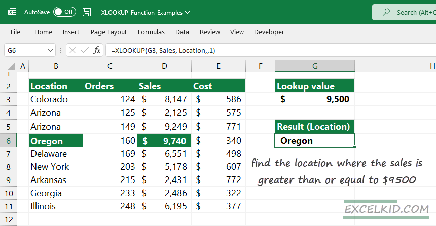
XLOOKUP does not find an exact match, so it will use the next larger item as a lookup value, in this case, 9740.

Formula:

=XLOOKUP(H3, Sales, Location,,1)

Result: the corresponding item based on the lookup value: Illinois.

If you want to learn more about this feature, here is a more advanced example of the approximate match to find the closest match in an array.

Wildcard character match (* or ?)

We’ll show you how to use the XLOOKUP wildcard search function in the following example.

We aim to look up the location that begins with “DE” and return the sales. Use “*” for any number of letters. Set the 5th parameter of the XLOOKUP function to 2 if you are using wildcard character search.

• lookup value: = G3&”” = De*
• lookup array = Location
• return array = Sales
• match mode = 2

Formula:

=XLOOKUP(G3&”*”, Location,Sales,,2)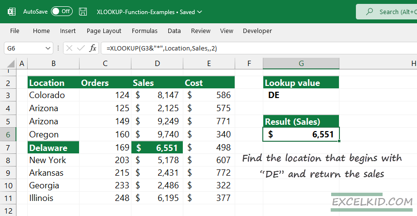

Sometimes you want to replace a single letter in a word, use the “?” symbol. We use the wildcard search, so don’t forget to use 2 as a parameter for the match mode argument.

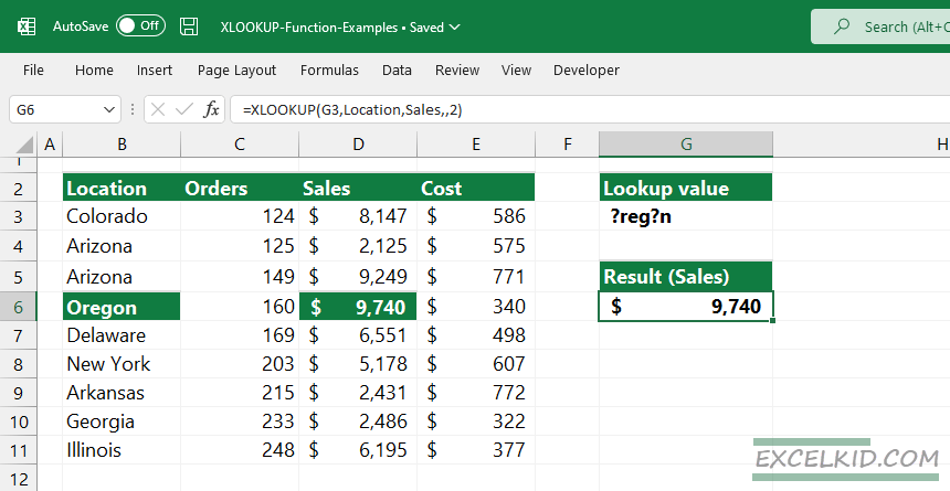
Formula:

=XLOOKUP(G3, Location, Sales,,2)

Here is a detailed example of how to return the last match in a range in case of an exact match.

XLOOKUP last to first search mode

The following two examples will explain how to use the search_mode argument of the XLOOKUP function in Excel.

In the first example, we’ll use two optional arguments for XLOOKUP to specify the match type (0 is for exact match) and match direction (-1 is for the bottom to top).

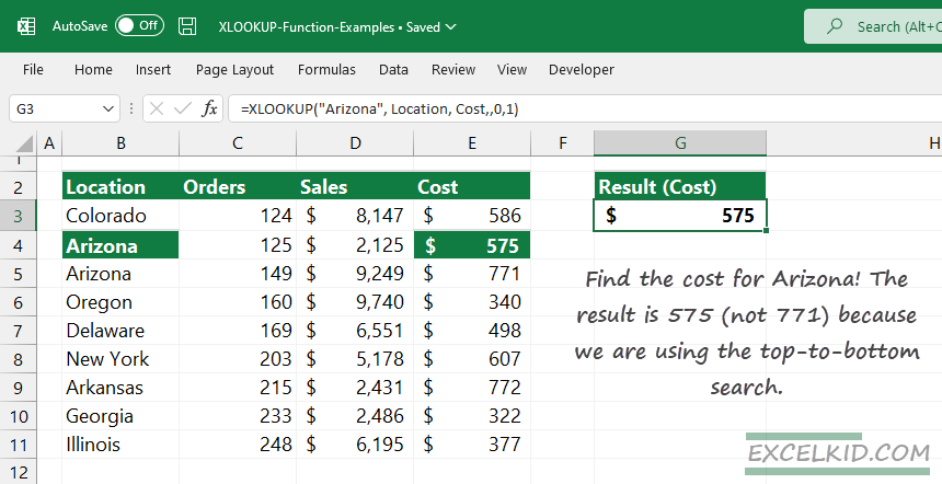
We aim to find the sales for “Arizona” using the last-to-first search mode.

Formula:

=XLOOKUP(“Arizona”, Location, Cost,,0,-1)

We use two (5th – match mode argument and 6th – search mode argument) of the three optional arguments. Parameters are comma-separated-values, so if the 4th parameter is not necessary, type a comma, then add the 5th and 6th arguments to XLOOKUP.

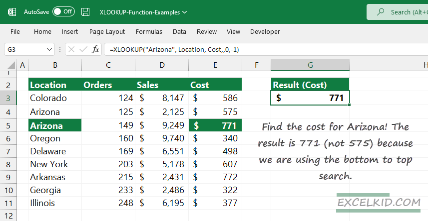
Reverse search starting with the last item. The result is 771 because we are using the bottom-to-top search.

XLOOKUP first to last search mode

Now, let us see what will happen if we use the bottom-to-top search. Our goal is to same as the example mentioned above: find the matching record in the “Cost” column where the location is equal to “Arizona”.

Formula:

=XLOOKUP(“Arizona”, Location, Cost,,0,1)

In this case, we use “1” as the 6th argument.

Explanation: The formula searches for the first matching value in the range ‘Cost’. The result is 575 (not 771) because we use the first-to-last search mode.

Binary search

A binary search can be faster than a linear search if you work with a huge array and your data set is sorted. Let us see the workaround with binary search lookups. In the picture below, we try to find the lookup value in an unsorted array using binary search.

In the example, we want to find the matching value in a Sales column for the lookup value, “Oregon”. First, make sure that the search_mode argument = 2.

Evaluate the formula:

=XLOOKUP(G3, Location, Sales,,,2)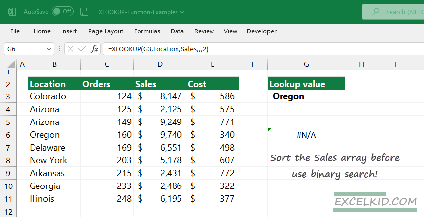

The result is an #N/A error. To avoid this type of error, ensure your array is sorted. In this example, you must apply a sort to get the Sales column items in ascending order.

Learn more about binary search.

XLOOKUP multiple results

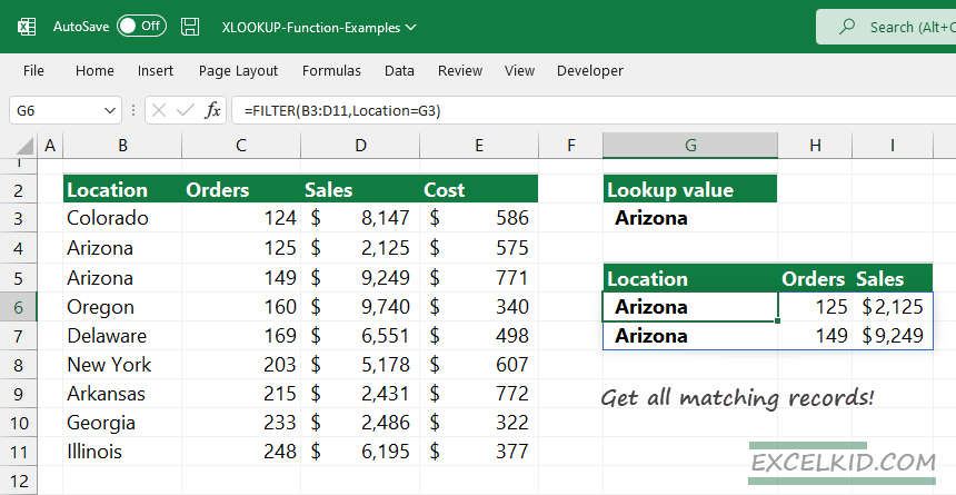
What if we have multiple matching records? Is it possible to get all matching records using XLOOKUP?

In the example, we want to list all sales records where the location = ‘Arizona’. Therefore, use the FILTER function instead of XLOOKUP on the data set.

Then, enter the formula in cell G6:

=FILTER(B3:D11, Location=G3)

Excel automatically spills the results into adjacent blank cells.

Why XLOOKUP is better than other lookups (VLOOKUP, HLOOKUP, INDEX, and MATCH)

Key advantages of using XLOOKUP:

1. XLOOKUP reduces formula errors: Type XLOOKUP(value_to_find, where_to_find, the result list) and job done. The formula returns with a #N/A error if the value is not found.
2. XLOOKUP handles left lookup problems and replaces the VLOOKUP function + CHOOSE workaround.
3. Returns exact match by default. The last argument is the most frustrating thing about using the HLOOKUP and VLOOKUP functions. You have to use FALSE to get the correct result. On the other hand, XLOOKUP returns with the exact match by default.
4. The function is not case-sensitive by default. Here is the workaround to get case-sensitive values.
5. XLOOKUP supports a 4th parameter: the “value not found” scenario. From now, error handling will be much better. Instead of using IFERROR, IFNA, or other error-handling functions, you can add the default output if the value is not found.
6. The 5th argument supports the approximate match.
7. It uses an optional 6th argument for special searches and supports wildcard, top, and bottom searches.

XLOOKUP Formulas

Additional resources:

I hope you can find helpful our definitive guide. If you want to expand your knowledge, we strongly recommend the following list. These articles are for advanced Microsoft 365 users. Using these examples, you can do almost everything regarding lookups. All formula examples contain a downloadable Excel Workbook.

1. How to use logical criteria as a lookup array
2. Spill matching values into rows and columns instead of single cell
3. How to lookup values across multiple Worksheets
4. Learn how to find the 2nd, 3rd, or nth match in a range.
5. Find the nth largest value in a range
6. Lookup the first negative value in a range
7. Get the first text value in a range
8. How to perform a nested (two-way) lookup in case of multiple variables
9. How to lookup values between two numbers
10. Find the first or last positive value in a list
11. Return the nth value using NVLOOKUP

Have you problems with the function? Take a closer look at the next chapter.

Why is XLOOKUP not working properly?

In this chapter, read the definitive guide on fixing your formula if it is not working.

XLOOKUP provides almost endless possibilities in Microsoft Excel. But the function in some circumstances brings difficulties. When the XLOOKUP is not working with your Excel version, please read our guide, and check the possible workaround and fixes.

Take a closer look at the list below! Here are the top five reasons why your function is not working. Look at your formula error and jump to the given section:

1. XLOOKUP is not supported
2. #VALUE error
3. #N/A error
4. #NAME error
5. #SPILL

1. XLOOKUP does not appear or is not supported

XLOOKUP is only part of Microsoft365 subscriber licenses; ensure you use the correct version. If you have a recent Excel version, use an add-in that implements the function.

It is easy to check your Excel version. First, click File > Account and look at the product information window. If your Excel version is not supported, please do not panic. Instead, use our add-in. It is fully compatible with all recent Excel releases.

2. #VALUE errors

Fixes Different array sizes using the TRANSPOSE function

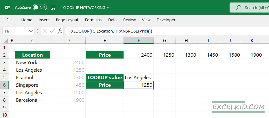
In the example, you want to use the lookup function and find the correspondent record for Paris. Location and Price are named ranges referred to as C3:C8 and range F2:K2. The function will return a #VALUE error because the Location array size is 1×6 and the Price array size is 6×1.

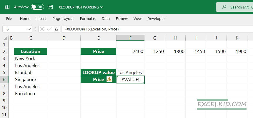
To fix the formula, use a TRANSPOSE function and convert the Price range to a column. I inserted the transposed “virtual array” in column D to make this example easy to understand.

Row size differences

XLOOKUP is not working properly if you use different row or column sizes. For example, the lookup array (C3:C8) contains six rows, but the return array (D3:D7) has only five rows. The array’s size difference is why the #VALUE error appears in cell G7.

It’s easy to check your setup. But first, you should have to click on the Formula Bar.

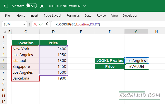
Excel will highlight all arrays. First, you must add the last row in column D in the lookup array. After that, the formula will return the estimated value.

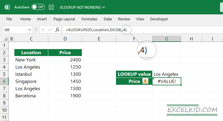
Function Argument is not valid

As we know, the function uses three required and three optional arguments. Here are the possible values for the 5th and 6th arguments:

• match mode: {0, -1, 1, 2}
• search mode: {1, -1, 2, -2}

Look at the formula below! We are using “4” as match mode. Because it is not valid, we’ll get a #VALUE error.

3. #N/A errors

The main reasons for getting #N/A errors:

• No exact match
• No approximate match
• Numbers stored as text
• The lookup array is not sorted
• The formula contains unnecessary or extra characters

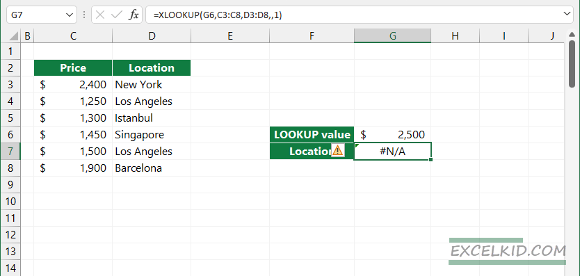
Missing error handling in case of no exact match

If you are not using the match_mode argument, XLOOKUP looks for an exact match. If the function does not find the lookup value in the lookup array, the formula will return the #N/A Error.

To avoid these errors, use a custom text for error-handling purposes (like “value not found”).

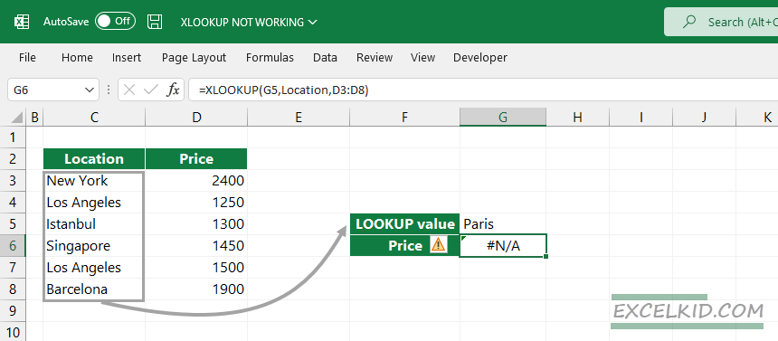
No Approximate Match

In the example below, set the match_mode to 1. Then, the function tries to find an exact match. In case of no exact match, it will return the next largest value from the lookup array greater than the lookup value.

We have no exact match, and if all values in the lookup array are less than the lookup value, the function will return an #N/A error.

When XLOOKUP is not working, try to use the 4th argument to handle errors, and the formula will return an easily understandable message.

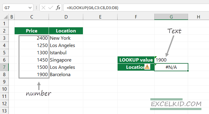
Different Data Types

The most important rule:

lookup value data type = lookup array data type

For example, if your lookup value is a number, the function will work only if the lookup array contains numbers. In the picture below, our lookup value looks like a number. No, not that all. In cell G7, we have a number that Excel store as text.

We have to apply a quick conversion. To do that, apply these steps:

• Select the cell that contains the lookup value
• Locate the triangle icon on the top-left corner of the cell
• Use the Convert to Number option

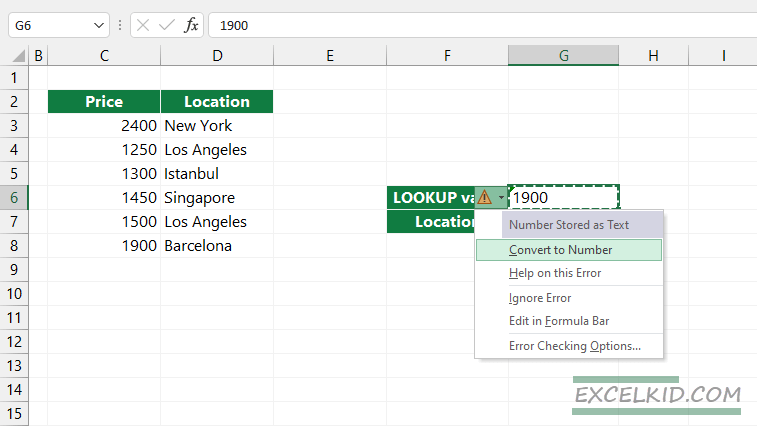
Your function will work again!

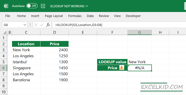
Unwanted characters in lookup arrays

Working with formulas is easy, but sometimes you have a non-printable or unwanted character in the lookup or return arrays. These characters, like spaces, do not make your life easier.

In the example below, everything looks great, but we get an #N/A error even if the lookup array contains the lookup value.

What might be the problem with the formula? In this case, it is worth using the LEN function to check the array integrity. Hint: the C3 cell contains two extract spaces, so “New York “ is not equal to “New York“.

The good news is that we can clean the data on the fly using the TRIM function.

Here is the solution:

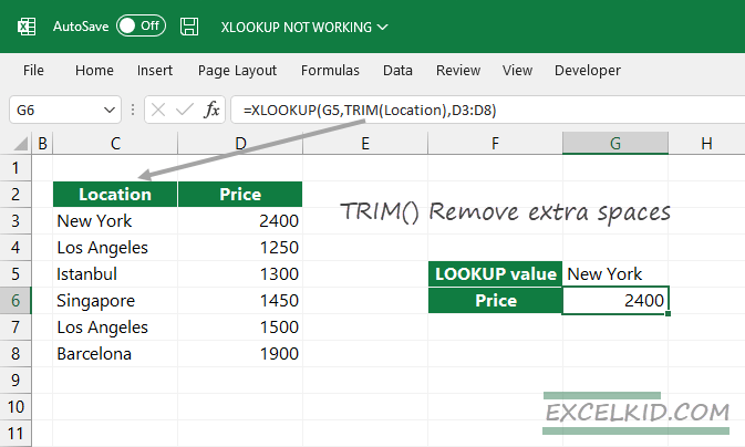
Our formula now works fine!

Unsorted records in the lookup array

In the following example, you use -2 as the 6th parameter to lookup a value in a lookup array. Good to know that the binary_search parameter requires a sorted array.

To solve this tiny but frustrating problem, you have two ways:

• manually sort the records in the array
• using the SORT and SORTBY function

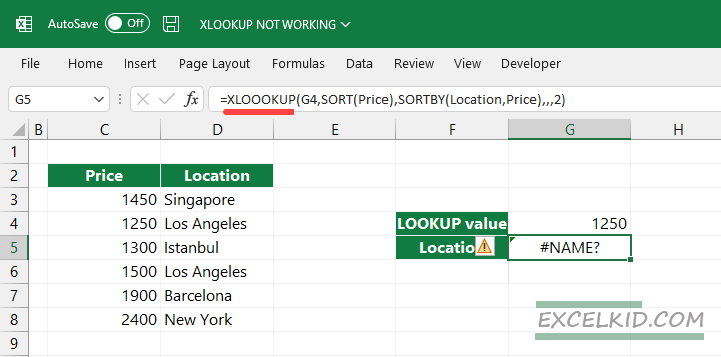
In this guide, we’ll explain the function-based solution:

=XLOOKUP(G5,SORT(Price), SORTBY(Location,Price),,,2)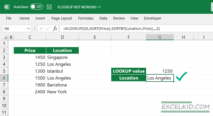

Both functions sort the selected arrays using ascending orders. The main difference between SORT and SORTBY is:

• SORT returns with an array
• SORTBY returns with a part of an array; in this case, the Price column

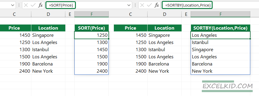
Both functions create a dynamic array for the lookup_array and return_array.

4. #NAME errors (typo, human errors)

The #NAME error may appear in the following cases:

• Typo with names
• Missing or incorrect usage of named ranges
• Comma or semicolon issue

The function has a typo

We added XLOOOKUP instead of the proper function name in the formula example.

The formula in cell G5 will return an #NAME error.

Missing or incorrect usage of named ranges

At first look, the formula looks correct, but it returns an error. First, make sure that the named range exists! It is easy to check whether the named range is valid or not.

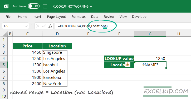
Locate the Formulas Tab on the ribbon. Click Name Manager! You can review all named ranges in the worksheet or the complete Workbook. Because “Location” <> “Locations”, it causes #NAME errors.

Comma or semicolon issue

When your XLOOKUP is not working, consider the correct separator between function arguments. Comma or semicolon? It depends on your Excel version.

Good to know that only the US English version of Excel uses a comma (,) to separate arguments. International versions use a semicolon (;) by default.

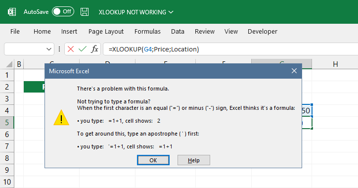
We use the US-English version of Microsoft Excel in the example, so we’ll get an error. To fix it, use a comma to separate the arguments.

5. #SPILL

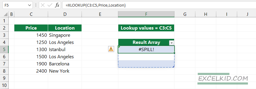
You frequently faced the #SPILL error. The main cause: the result array can not overwrite other cells if there are not blank.

The output array contains data

You want to use multiple lookup values in the example, and the function works fine. The result is an array!

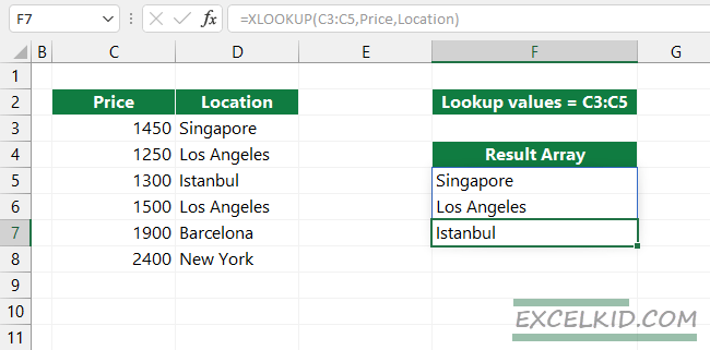
What if one or more possible output cells contain text values or numbers?

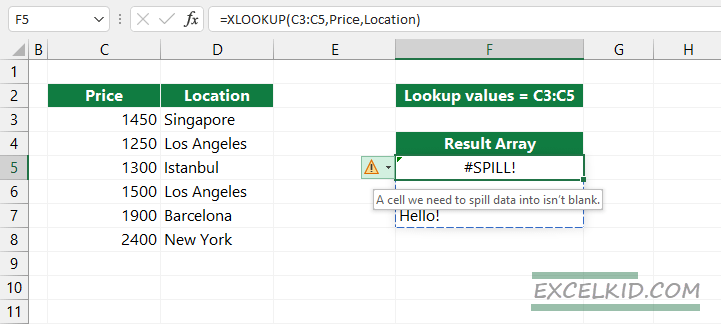
Move the mouse over the yellow triangle. The error message is: “A cell we need to spill data into is not blank”.

Excel Table does not support dynamic array formulas

In the example, you use an Excel table with multiple lookup values. Don’t do that.

Tip: Instead of using multiple lookup values, use a single value; Excel will copy the results until the end of the table without getting an error.

Thank you for being with us today; we hope this guide was helpful and your formulas will work fine. Stay tuned and follow our latest function guides and tutorials!

Additional resources

• Excel Formulas
• Excel Functions
• Formula Errors