Learn how to get the last match in a list or a range using the ‘last to first’ search of the XLOOKUP function.
XLOOKUP is a multipurpose function that enables you to perform advanced lookups. Today, we will show you an easy example.
Example: Get the last match using XLOOKUP
In a nutshell:
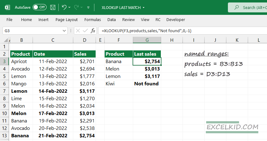
If you want to extract the last match in your list or range, use -1 as the fifth argument of XLOOKUP.
To make the formula easy to read, use named ranges! For example, select the range B3:B3, locate the name box, and type ‘Products’. Next, use the ‘Sales’ for range D3:D13.
Enter the simplified in cell G3. The formula looks like this:
=XLOOKUP(F3, products, sales,”Not found”,0, -1)
Let us see the arguments:
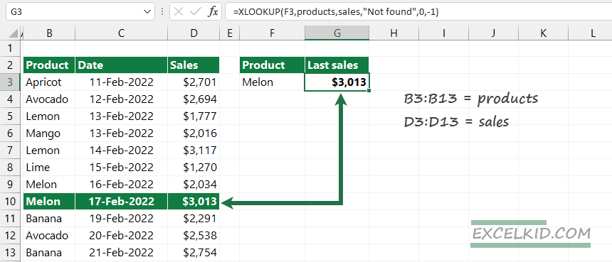
- lookup_value is F3, “Melon”
- lookup_array is a named range, B3:B13, “Products”
- return_arry is a named range, D3:D13, “Sales”
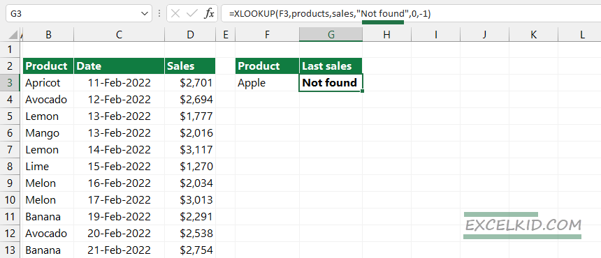
- not_found is an error-handling argument, if no match, return the “Not found” text string
- match_mode is 0, looking for an exact match
- search_mode is set to -1 (last to first search)
How the search_mode works
XLOOKUP returns the first matching record if you are not using the 6th argument. You can configure the search_mode argument and control the search direction.
To change the default search mode to “last to first”, – start the search from the bottom- use the -1.
Starting from the bottom, XLOOKUP tries to find the lookup value, in this case, “Melon”. In cell B13, nothing is found. So, the formula evaluates the next row. In the case of an exact matching record in column B, the function returns with the corresponding sales in column D.
You can use the 4h argument for error handling if no match is found. (If you are not using the error-handling argument, XLOOKUP will return an #N/A error.
=XLOOKUP(F3, products, sales,”Not found“,0, -1)
Additional resources:
Related formulas: