Learn how to find the closest match in numeric data quickly using the XLOOKUP function or INDEX and MATCH combinations.
Finding the closest match in Excel is a real challenge! Everyone knows that the XLOOKUP function is a Swiss knife, so we’ll use the 5th argument (match mode) in the example. In the second part of the guide, we’ll combine the main function with the ABS function to get the closest match. The million-dollar question: is the “next larger item” or the “next smaller item” the closest? Not at all!
How to find the closest match in Excel
Here is our table, which contains two columns: Location and Price. For the sake of simplicity, we use named ranges.
- Location: B3:B12
- Price: C3:C12
Find the next smaller item (or exact match)
In the first example, we try to find the closest match and set the 5th argument to -1.
The arguments look like this:
- lookup value: F4
- lookup array: Price
- return array: Location
- match mode: -1
Formula:
=XLOOKUP(F4, Price, Location,,-1)
Tip: If you need to skip one or more optional argument(s), type a comma between the arguments; the function will not use it. We do not use the “if not found” and “search_mode” arguments in the example.
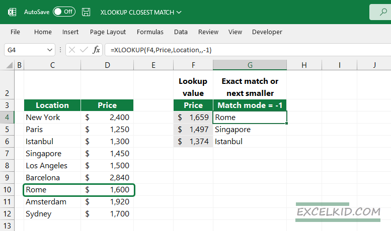
The result is Rome. Okay, take a look at how the formula works. First, Excel evaluates the formula and uses the lookup value ($1659) to find an exact match. If an exact match is not found, it returns with the next smaller item, in this case, $1600. Finally, the formula returns with the corresponding Rome record in the example.
Find the next larger item (or exact match)
In the following example, our goal is the same, but we’ll try to find the closest match using another value for match mode.
Evaluate the formula:
=XLOOKUP(F4, Price, Location,,1)
The formula returns with “Sydney” if you use the F4 cell as a lookup value and set the match mode argument to 1. If an exact match is not found, it returns with the next larger item, in this case, $1700. Finally, the formula gets the corresponding value in the Location column, Sydney.
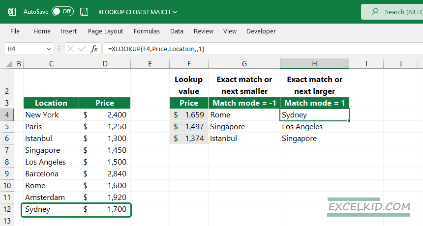
We had different results in case no exact match was found.
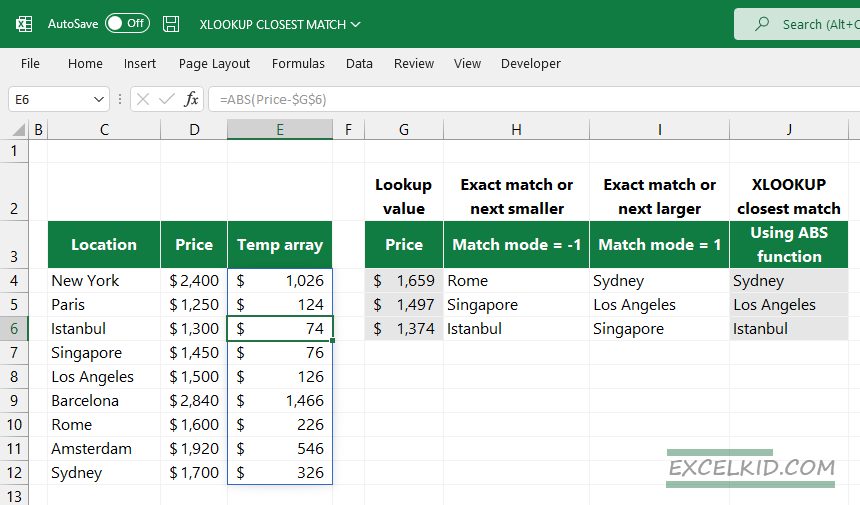
Solve the closest match challenge: XLOOKUP and ABS function
Now, here comes the moment of truth! If you want to find the closest value, you must use the ABS function.
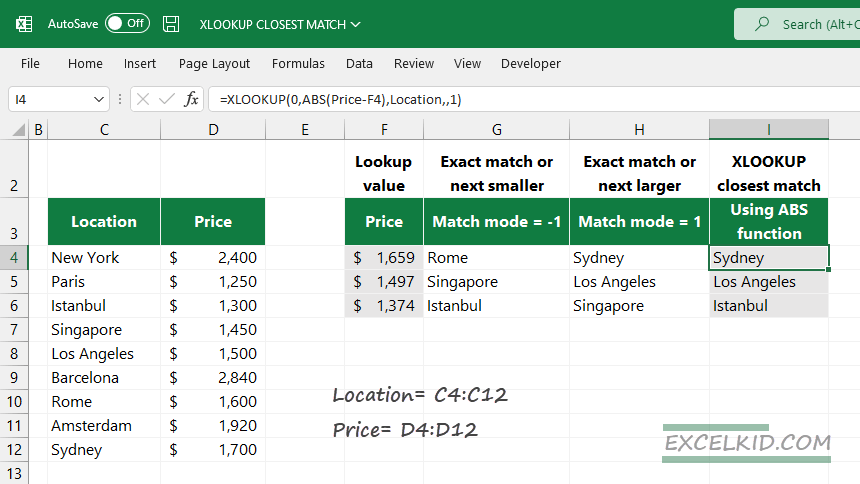
Please look at column J! First, let us see the formula, and then we’ll explain how it works.
=XLOOKUP(0, ABS(Price – lookup_value) ,Location,,1)
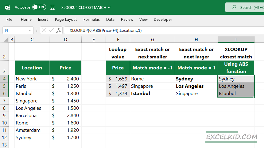
Evaluate the formula in J4 from the inside out:
=XLOOKUP(0, ABS(Price-G4), Location,,1)
- lookup value = 0
- lookup array = ABS(Price – lookup_value) – it creates a new dynamic array with calculated values
- return array = Location
- match mode = 1
The lookup value is 0, so the formula tries to find the closest value to 0 in column E’s newly created temporary array. The closest value is $41, and the corresponding value in the same row is Sydney.
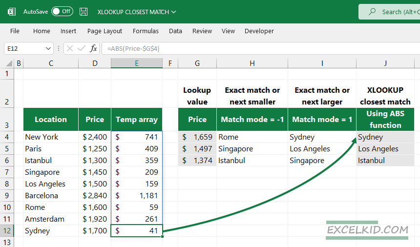
The formula in cell I5 works the same; the result is Los Angeles.
Finally, evaluate the formula in I6 from the inside out:
Finally, here is a quick summary! The demonstrated method finds the closest value without any trouble.
Workaround with INDEX and MATCH
Here is a workaround with the INDEX and MATCH functions. The task is the same. Again, try to find the closest match if you have a recent Excel version.
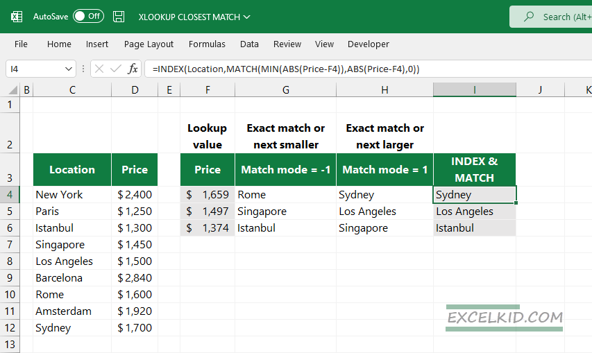
Formula:
=INDEX(Location, MATCH(MIN(ABS(Price-F4)), ABS(Price-F4), 0))
- MIN function finds the smallest differences
- ABS function converts the negative value to a positive
- MATCH returns the position in the array Price
- INDEX returns the correspondent value in the Location array