How to use Conditional Formatting

Conditional formatting is a data visualization tool in several spreadsheet applications. We use it to highlight, emphasize, and differentiate by using colors or other means (like applying icons) to cells or ranges relevant to us.

At first, you will learn the essential skills. The second part of the tutorial will be about using Excel conditional formatting formulas and examples.

Table of contents:

1. What is Conditional Formatting
2. Learn the fundamentals of Conditional Formatting
3. Highlight cells
4. Highlight cells that contain text
5. Edit a conditional formatting rule
6. Delete a conditional formatting rule
7. Conditional Formatting Formulas: Examples

What is Conditional Formatting

Conditional formatting offers a wide range of possibilities for Excel users. Its first and foremost function is to direct attention to the most crucial data points. Then, we can determine with rules what are the most important for us. These data points can be deadlines, excellent sales results, or tasks carrying a high risk.

Download the practice file!

Fundamentals of Conditional Formatting

Before we walk you through all possibilities of conditional formatting, we have to stall a bit. It is necessary to know all the basics! First, you have to understand the structure that conditional formatting provides. So, let’s see a little overview. In short, we will summarize the most important rules for you.

Logical Operators (if-then rules): Every single conditional formatting rule is based on straightforward logic. If “X” criteria are true, then apply the rule “Y”. Let’s see a simple example: “X” criteria are: “The sales price is more than $50.” “Y” criteria are defined as a color all applicable cells red. What will happen now? By applying the if-then rule, every cell will be colored red where the sales price is > $50, more than $50.

Predefined Conditions (built-in presets): This option can interest beginners. In Excel, there are many built-in rules and conditions available. We have also thought about users with different capabilities when making the tutorial. We will learn about this subject from a detailed guide.

User-defined Conditions: There are often situations when the default settings are unsuitable for the given task. No problem, let’s make our own rules. Use the Excel formulas so we can reach the required results. We have to note that we can use all of the formulas in Excel to create the rules.

Multiple Conditions: We can simultaneously apply multiple rules for one cell or range. If there are more rules active simultaneously, which one will prevail? We will discuss this in detail in the chapter “rule hierarchy and Precedence.”

Highlight Cells using rules (if the quantity is greater than 200)

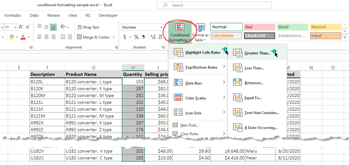
Click the Highlight Cells Rules functions to highlight patterns and trends with conditional formatting. It will be straightforward to identify the cells that meet your criteria. This is a basic color formatting method for cells and ranges.

Select the range you want to use a rule and apply highlight rules. In our example, we will highlight any product that’s quantity is greater than 200 units. For example, select the range’ H2: H24‘.

In the Home tab of the ribbon, click Conditional Formatting, then click Highlight Cell Rules. Finally, select ‘Greater than’.

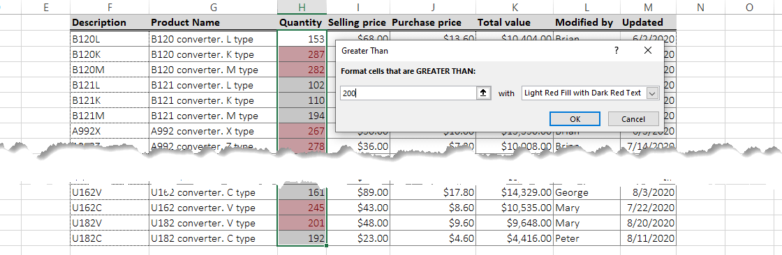
Now, a dialog box will appear. Enter 200 In the left box. So, if you enter 200, something will happen when the value is greater than 200. But what will happen? You will define the trigger in the right box.

Explanation: Triggers can be defined in the range with which the event is associated. Remember the standard option and select a light red fill from the drop-down list. If you click OK now, all the cells that are above 200 will be formatted based on the given rule.

Highlight cells that contain text

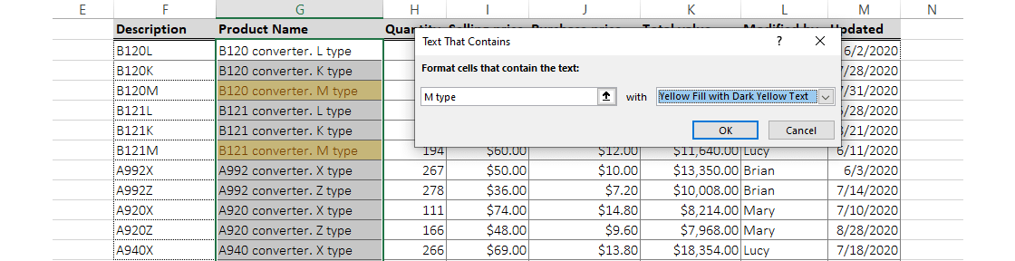
If you are looking for all the M types of converters in column G, you do not have to scan the screen for hours and hours. Instead, you can let conditional formatting do all the dirty work and highlight the criteria easily and automatically.

Select the range with text. In this example, you will select the range G2:G24, all our ‘Product Name.’

Click Conditional Formatting, hover the mouse over Highlight Cells Rules, and choose Text that Contains.

Enter “M type” in the text box. Next, select yellow fill color with dark yellow text using the drop-down menu, then click OK.

Tip: You can apply a custom format if the default style is unsuitable. Use the drop-down menu and select the Custom format option to create your format. You can create custom styles by changing the font, border, or fill types. Keep in mind the basics of conditional formatting! Further options are available if you can apply different rules.

You can also use important highlight rules for your values: Greater than…, Equal to…, or Between.

Editing a conditional formatting rule

This section will show you how to manage conditional formatting rules. You can modify the selected rule using the conditional formatting rules manager. Use this function if you want to edit some of these rules later or delete them.

This function can be accessed using the Home Tab and the Conditional Formatting button. Then select Manage Rules from the drop-down list. By default, you’ll see a dialog box:

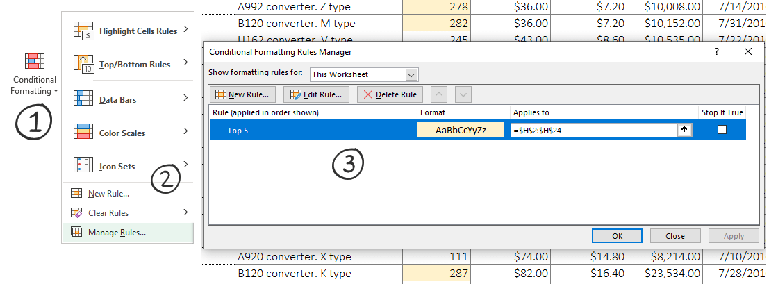
By default, the “Show formatting rules for:” is set to “Current Selection”. Next, select the “This Worksheet” option from the drop-down list to display the conditional formatting rules you have applied to the actual Worksheet.

Use top-bottom rules and select the rule from the list you want to modify. Then, click the rule you want to change to edit a rule. In this example, we want to highlight the top 10 values in the Total value column. Currently, the top five are highlighted.

Click the Top 5 rows! Excel highlights the selected rows with blue. Then, click Edit Rule. A dialog box opens where you can change the given conditions of the rule; type 10 in the number field. Finally, click OK.

We’ll get the Manage Rules box back. Click OK to save the changes.

Delete a conditional formatting rule

Sometimes your spreadsheet looks like a traffic jam regarding too many conditional formatting rules. This is because Excel has a hidden “feature.” If you have many unique rules, that may be the reason for the slow calculations. In this case, you should eliminate some rules in the sheet.

Tip: Excel provides a quick way to delete rules. Click the Conditional Formatting button on the Home tab and select clear rules.

But it’s not smart to delete all rules from a worksheet!

In this case, we want to delete the rules from Column G (Product Names). Select the ‘G2:G24’ range.

To properly delete a rule, select the ‘Manage Rules’ box and click on the conditional formatting rule you want to remove.

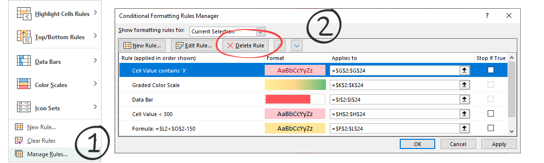
Click OK to delete the rule.

We hope you have found the first part of the tutorial interesting and exciting. In this, we have introduced how we can use the basic rules with Excel.

Conditional Formatting and Formulas

You’ll find here 50+ formula examples and learn more about custom formulas.

All examples are based on a few simple steps:

1. Select the range that you want to apply the format
2. Add ‘New Rule’
3. Enter the formula
4. Select format style
5. Click ‘OK, then click ‘Apply.’

That’s all.

Check our definitive guide with examples if you want to learn about Excel Formulas.

How do I highlight the lowest 3 values in Excel?

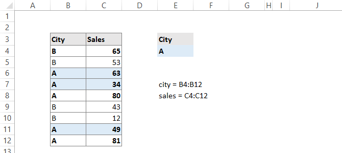
Create a formula to determine the 3 smallest values that meet specific criteria. Use a formula based on the AND and SMALL functions. In the example, the formula used for conditional formatting is:

=AND($B4=$E$4,$C4<=SMALL(IF(city=$E$4,sales),3))

where “city” is the named range B4:B12, and “sales” is the named range C4:C12.

How to use conditional format if the cell is blank?

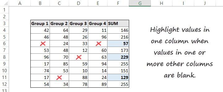
In the following example, you want to highlight values in one column when values in one or more columns are blank. A basic formula based on the OR and ISBLANK functions is used to test for blank or empty cells. For example, if any cell in a corresponding row in the range B4:E12 is blank, OR function returns TRUE. Thus, the trigger will be fired, and the cell in column F will highlight using light blue.

Use the conditional formatting formula:

=OR(ISBLANK(B4),ISBLANK(C4),ISBLANK(D4),ISBLANK(E4))

How to use Conditional Formatting to highlight past due dates in Excel

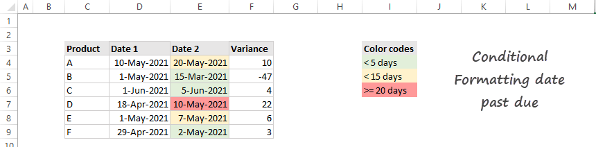
You will apply a formula in the example to determine “past due dates.” The formula will check if the variance between dates exceeds a certain number of days. To create a color-coded table, use three conditional formatting rules for each interval.

Select the cells in range E4:E9 and apply the formulas.

1. =(E4-D4)<5 if the variance is less than 5 days,
2. =(E4-D4)<15 if the variance is between 5 days and 15 days
3. =(E4-D4)>=20 if the difference between the two dates is greater than or equal to 20

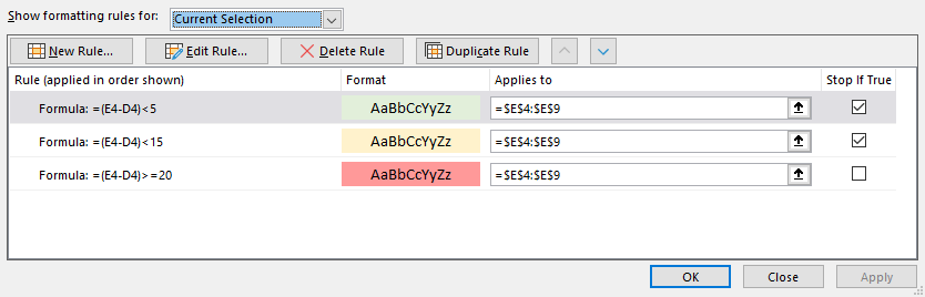
Important: You must use the stop-if-true checkbox for rule 1 and rule 2.

How to highlight overlapping dates in Excel

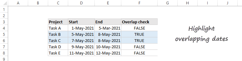
Sometimes you need to highlight cells where dates overlap. You can use conditional formatting formulas and apply the SUMPRODUCT function in the example. What are overlapping dates? We are talking about overlapping dates if these two conditions are true:

1. First, the start date is less than equal to the other end dates in the column.
2. The end date is greater than or equal to at least one other start date.

Create a new column to check the conditions. Then, apply the formula to cell F4 them copy the formula down.

=SUMPRODUCT(($D4<=$E$4:$E$8)*($E4>=$D$4:$D$8))>1

Result:

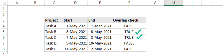
Now create a conditional formatting rule. First, select the cells you want to format, in this case, range C4:F8. Then use the rule below to highlight overlapping dates.

=$F4=TRUE

So, click OK to apply the rule. If the result is TRUE, the given row cells in the selection will be highlighted.

Advanced Guide to Mastering Conditional Formatting in Excel

Conditional formatting in Excel is not just about highlighting cells; it’s about unlocking a new dimension of data analysis and presentation. By understanding its deeper functionalities and integrating it with other Excel features, users can achieve unparalleled insights into their data.

Advanced Conditional Formatting Techniques

1. Data Visualization Enhancements: Beyond basic color coding, conditional formatting can be used to create data bars, color scales, and icon sets that provide visual summaries of your data, enabling quick analysis and comparison.
2. Formula-Driven Formatting: Leveraging Excel formulas within conditional formatting rules can address complex criteria and scenarios. This includes highlighting duplicates, visualizing data trends, and even creating Gantt charts for project management.
3. Dynamic Ranges and Conditional Formatting: Utilizing named ranges or dynamic range formulas with conditional formatting can make your formatting rules adapt to changing data sizes, enhancing the scalability and flexibility of your spreadsheets.

Strategic Applications of Conditional Formatting

1. Risk Management and Error Identification: Use conditional formatting to highlight outliers, errors, or anomalies in your data. This is particularly useful in financial analysis, quality control, and any domain requiring precision and accuracy.
2. Project Tracking and Management: Conditional formatting can visually represent project timelines, status (e.g., completed, in progress, delayed), and priorities, making it an invaluable tool for project managers and teams.
3. Dashboard and Report Enhancement: Incorporate conditional formatting into Excel dashboards and reports to create dynamic, interactive, and visually compelling data presentations. This can significantly enhance the decision-making process by emphasizing key metrics and trends.

Integrating Conditional Formatting with Excel Features

1. PivotTables: Apply conditional formatting within PivotTables to highlight key data points, compare performance across different categories, or visualize data trends directly within your summarized data.
2. Excel Tables: Leveraging conditional formatting in conjunction with Excel Tables not only enhances visual appeal but also maintains consistency as tables expand or contract.
3. Excel Charts: While not directly applicable to charts, the data used to create charts can be conditionally formatted to highlight significant points, trends, or outliers, indirectly enhancing chart visualization.

Optimization Tips for Conditional Formatting

1. Managing Performance: Excessive use of conditional formatting, especially with complex formulas over large data sets, can impact Excel’s performance. Regularly review and streamline your rules, and consider alternative methods for very large datasets.
2. Rule Management: Utilize the Conditional Formatting Rules Manager to maintain an overview of all rules applied within a worksheet. This is crucial for managing rule precedence, editing existing rules, or troubleshooting unexpected formatting results.
3. Custom Formulas for Unique Scenarios: Don’t hesitate to craft custom formulas for conditional formatting. Whether it’s highlighting entire rows based on a single cell’s value or creating interdependent conditional formats across different sheets, custom formulas offer limitless possibilities.

Exploring Beyond Traditional Uses

1. Interactive Elements: Combine conditional formatting with Excel’s form controls (e.g., drop-down lists, sliders) to create interactive reports and dashboards that dynamically update based on user input.
2. Integration with Excel Functions: Advanced Excel functions, such as INDIRECT, SUMPRODUCT, and ARRAY formulas, can significantly expand the capabilities of conditional formatting, enabling highly specific and dynamic formatting rules.
3. Visual Project Schedules: Use conditional formatting to create visual representations of project schedules, timelines, and dependencies, mimicking Gantt chart functionality directly within Excel.

By embracing these advanced strategies and techniques, Excel users can transform their approach to data analysis and presentation. Conditional formatting is a powerful tool that, when fully leveraged, can illuminate insights, enhance productivity, and drive informed decision-making. Whether you’re managing data for business analysis, project management, or simply organizing information, mastering conditional formatting is a step towards harnessing the full potential of Excel.

Final thought

Finally, take a closer look at the advanced conditional formatting rules:

• You should know how the conditional formatting rule hierarchy works if you work with multiple rules.
• The Stop if True tool helps you to manage overlaps between rules.
• Color ranking helps you identify the maximum value in a range and highlight them.
• Learn how to use Multiple Conditions and Formulas.

Conditional formatting makes our lives in Excel a lot easier.

Use formulas wisely! We can highlight all the key information that fits the criteria. Knowing and applying conditional formatting rules decrease the time spent on data analysis. Therefore, we can be a lot more productive. We can effectively support company decisions by recognizing the patterns (whether positive or negative). Look at the in-depth article called ‘How to create an Excel Dashboard‘ regarding conditional formatting on our blog.

Additional resources

• How to use the Quick Analysis Tool
• Highlight every other row
• Compare two columns in Excel
• Build a Heat Map
• Change shape color based on cell value
• How to use data bars
• Apply colorful icon sets
• Color Scales
• Find duplicates
• How to use Conditional Formatting based on another cell
• Show protected cells