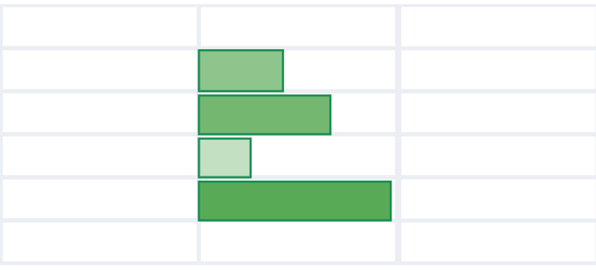
Data bars in Excel make it easy to highlight values in a range of cells. A longer bar represents a higher value. A shorter in-cell bar chart represents a lower value. Get a quick overview of highs and lows!
If you’re not using specific rules or conditions in your data range or cells, then data bars are great for showing the top or bottom values. We can apply it for the current selection (range or cell). It’s easy to visualize data using bars in Excel. This way is perfect for displaying the top-bottom values of your data.
To compare the values in the selected range, do the following steps.
Steps to create Data Bars in Excel
1. Select a range that contains your Data. First, we’ll apply data bars to range B2:B14.
2. Locate the Home Tab. In the Styles group, select Conditional Formatting.
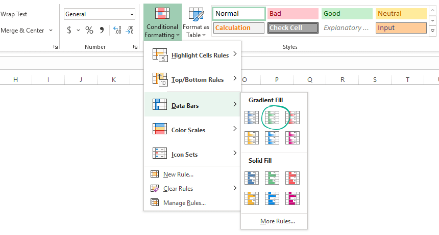
3. Click Data Bars. You have two options – Gradient Fill and Solid Fill. Select your preferred style. In this case, we will choose a gradient fill using green color.
Result:
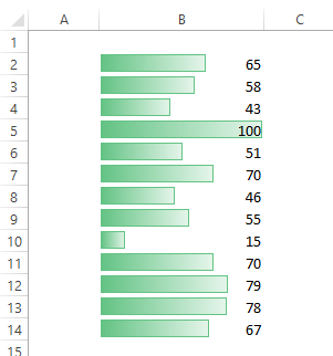
Explanation: In the example, we generated random numbers using the RANDBETWEEN() functions between 0 and 100. If you have a value that is less than zero, the data bar will not appear. In the range B2:B14, the minimum value is 0, and the maximum is 100. Between 1 and 99, all other cells are filled proportionally.
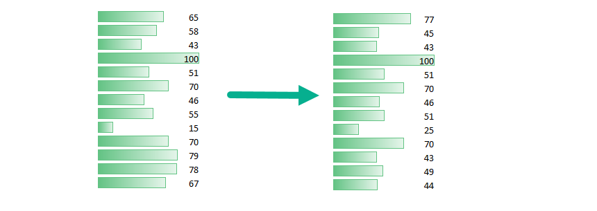
4. Change the values. Modify some values, and Excel updates the bars automatically.
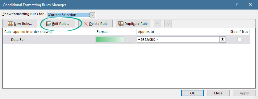
5. Select the range B2:B14.
6. Click on the Home tab again. In the Styles group, click Conditional Formatting, and choose Manage Rules. A new window appears.
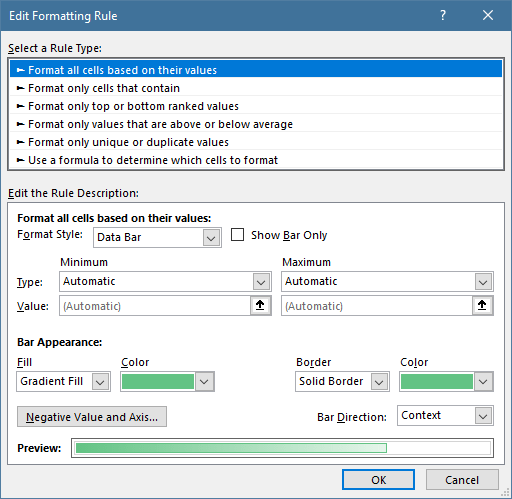
7. Click the Edit rule to start the Edit Formatting Rule dialog box. You can find here many useful options to customize your data bars. For example, you can show the bars only without displaying numbers. Change the default minimum and maximum values from automatic to Numbers, Percentages, or Formulas if you want to apply special rules.
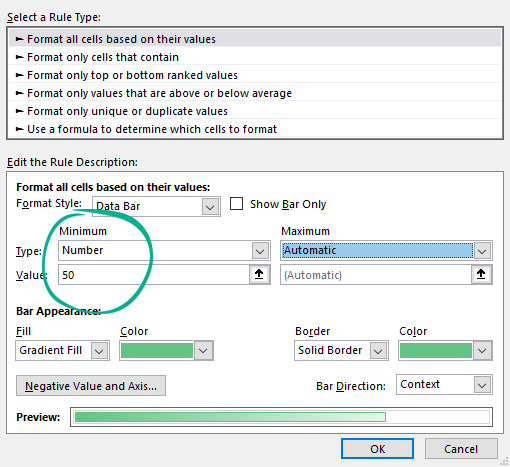
8. Select the Number from the Minimum drop-down list and enter the value 50. Leave the Maximum by Automatic.
9. Close the dialog box by clicking OK, and let’s see the result:
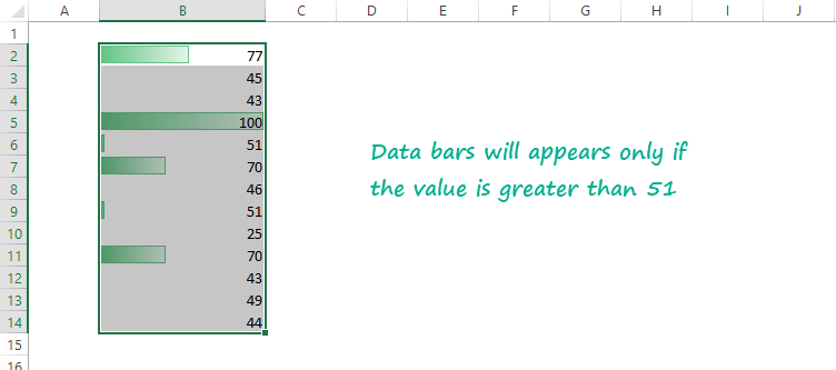
Explanation: the cell that shows a value that less than 50 has no data bar. Furthermore, the cell that holds a value that greater than 100 has a data bar that fills the entire cell. All other cells are filled proportionally.
if you want to learn more about conditional formatting, check the guide.