Icon sets in Excel are effective tools for us to visualize values in a range of cells easily. Each icon represents a range of values.
Execute the following steps if you want to add an icon set, shape, or indicator.
Steps to add Icons sets
We will use traffic light style shapes: green, yellow, and red traffic lights that indicate high, middle, or low values.
Step 1: Select a range that contains data
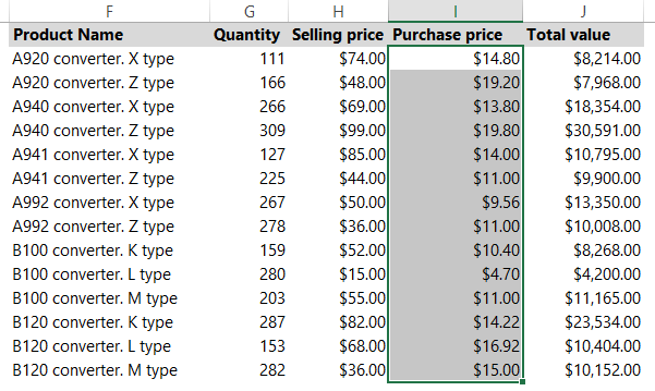
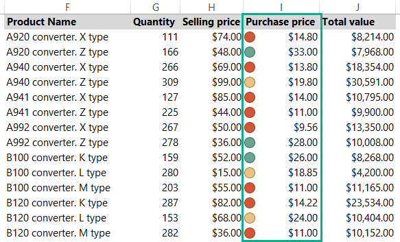
In the example, you want to apply icon sets to the column ‘I’ to highlight low, middle, and high-priced products.
Step 2: Go to the Home tab and select Conditional Formatting
Use the drop-down list to select Icons sets, then locate the Shapes Group.
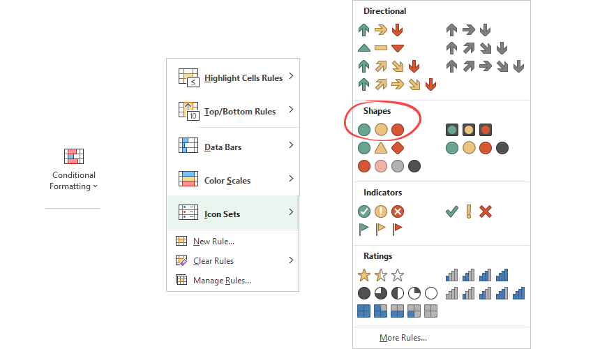
Step 3: Choose Icon Sets and click a subtype
You have various options for icons: Directional, Shapes, Indicators, and Ratings. Choose your favorite icon of these to fit the needs of your data.
Result:
Explanation:
By default, Excel calculates the green-yellow-red dividers for 67% and 33% for three shapes.
In this example, the minimum value is $4.70. The maximum value is $19.80
Above 67% (green shape) = min + 0.67 * (max-min) = 4.70 + 0.67 * (19.80 – 4.70) = 14.817
Below 33% (red shape) = min + 0.33 * (max-min) = 4.70 + 0.33 * (19.80 – 4.70) = 9.68
- A green shape will show values equal to or greater than 14.81.
- A yellow shape will show values greater than 9.68 and equal to or less than 14.81.
- A red shape will show values less than 9.48.
Step 4: Change the cell values
Let’s modify the values in the highlighted range! Excel will update the icon set in real-time.
Icon Sets Example
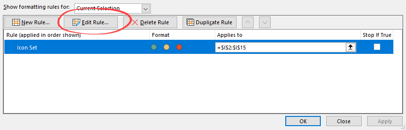
Select the range I2:I15
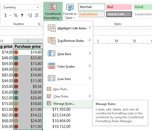
Locate the Home Tab on the Ribbon. Then, under the Styles group, click Conditional Formatting.
Choose Manage Rules!
Click the Edit rule:
Now you will see the ‘Edit Formatting Rule’ dialog box. Here you can change the icon styles and properties.
In the example below, you will change the formatting style. On the bottom-left area of the dialog box, use the drop-down menu to pick a new icon style, three traffic lights (rimmed).
Under the Type section, change the actual value to Number.
Apply the following rules: If the value is greater or equal to 17, you’ll see a green shape; between 13 and 17, apply red.
If the value is less than 13, you will use the ‘No Icon’ option.
Result: