
Learn how to combine the Excel RANK function and conditional formatting for color ranking and sorting purposes.
In the example, first, we want to create a sorted list using the RANK function. After that, we will highlight the top three products by sales using conditional formatting.
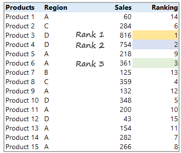
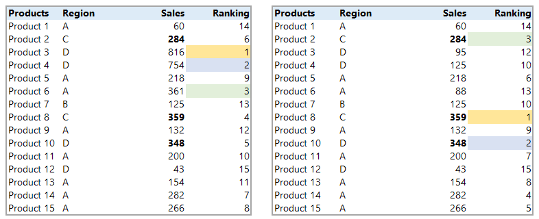
Our result is shown below:
But first, let us create a formula!
Color ranking using the RANK formula
How does the formula work?
The Excel RANK function returns a ranking of any number in the data (products, sales), and it is a built-in function in Excel.
We’ll apply two easy steps. At first, we’ll use the rank function to determine the sorting order (ranking).
The syntax is the following:
RANK( number, array, [order] )As you see, only two things and optional parameters necessary:
- The number is the value to find the rank for
- An array is the range of numbers that we will use for rankings
- Order is optional. We can decide the sort order (increase, decrease)
Steps to create dynamic ranking in Excel
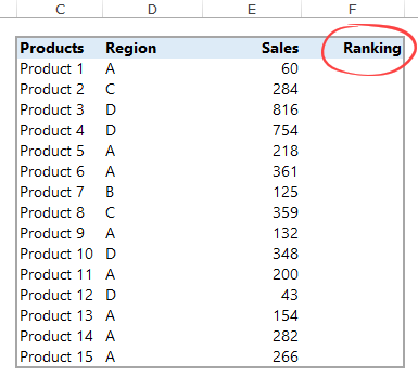
Step 1: Insert a new column for ranking:
Step 2: To rank the range E3:E17, select cell F3 and enter the formula below:
=RANK(E3,$E$3:$E$17,0)Copy the formula down until cell F17.
Result:
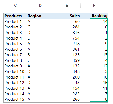
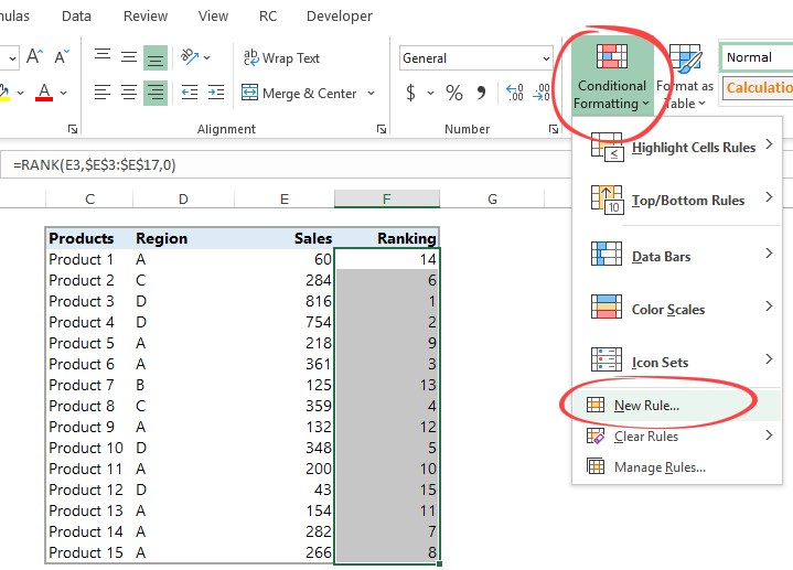
Step 3: Now, we have a list with ranks. Select the range!
On the Home tab, select Conditional Formatting. Next, choose the New Rule from the list.
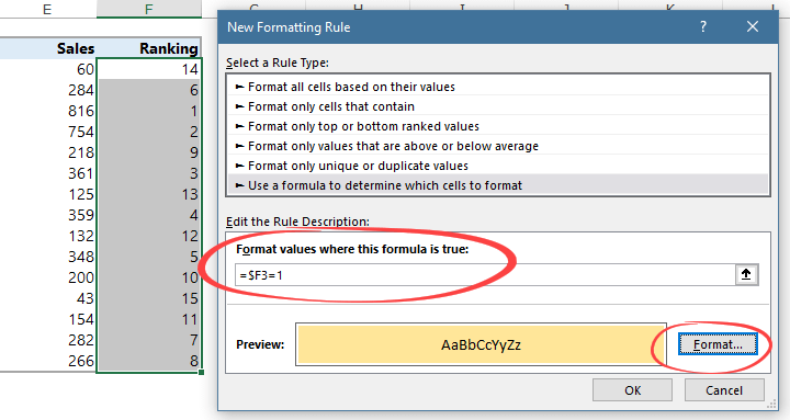
Step 4: A ‘New Formatting Rule’ window appears.
To add a new formula, select ‘Use a formula to determine which cells to format.‘ Under the ‘Edit the Rule Description‘, enter
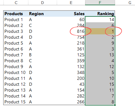
=$F3=1Because you want to use colors for ranking, choose a formatting style. Click Format and the Format Cells dialog will appear. In the example, we use yellow to highlight column E’s maximum sales.
Result:
Step 5: if you want to highlight the second, third, etc., highest value in a range and get the position, add new formulas to the highlighted range.
Use multiple rules and add =$F=2 for the second, =$F=3 for the third result.
The rule window looks like this:
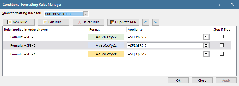
Click OK to add the second and third ranks.
Tip: The list is dynamic! If you change any values in column E (Sales), Excel will also change the rank and color.
Use color ranking to highlight the top n items in a range.
Additional resources: