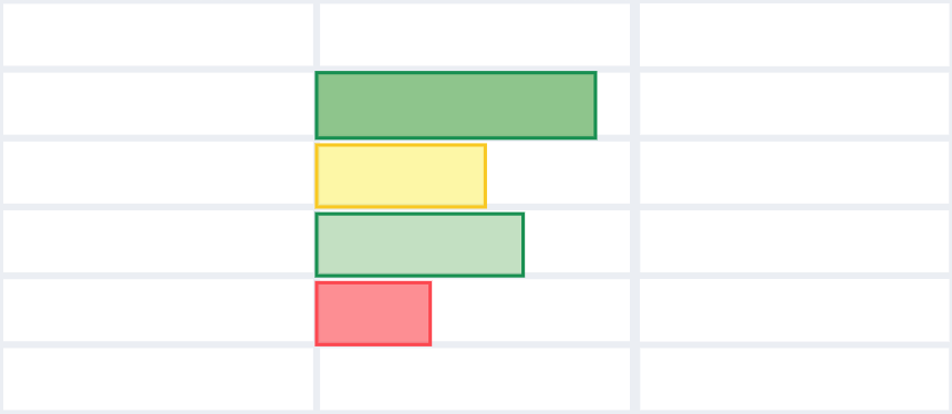
Color scales in Excel are similar to Data Bars. Get a quick overview of your data! The shade of the color represents the value in the cell.
Before taking a deep dive, you should know: What is the difference between color scales and data bars?
Data bars represent the relationship between value and colors through the length of a bar. Color scales assign colors to your range based on the selected scheme.
How to add Color Scales
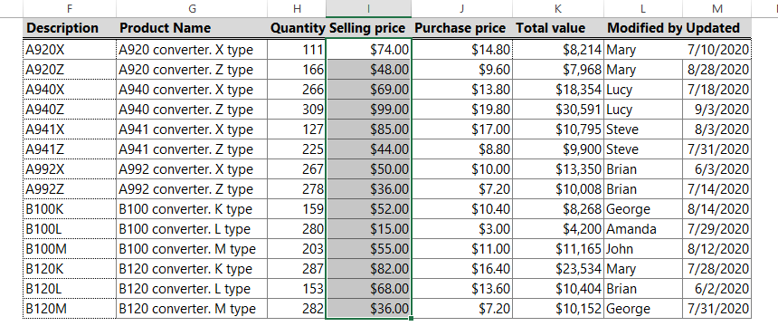
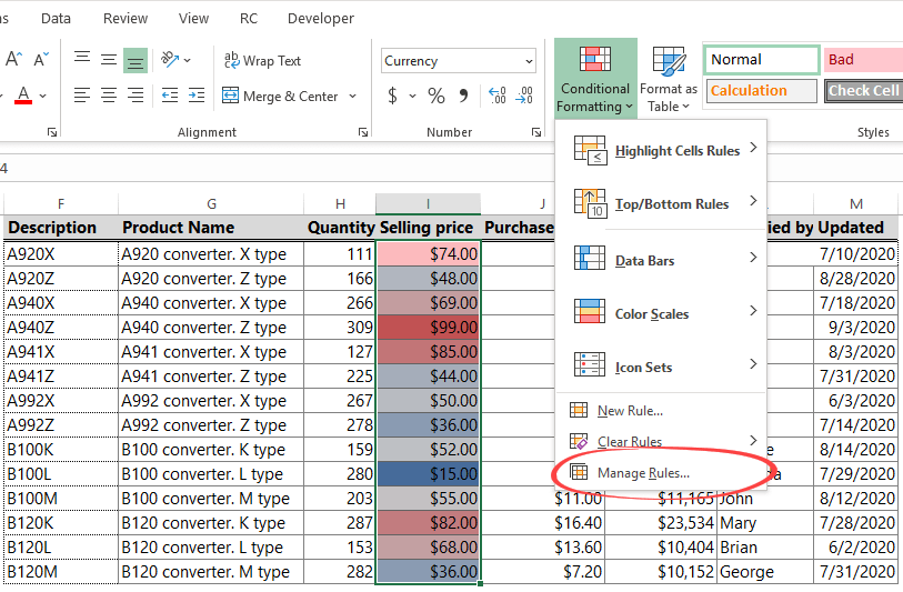
1. Select the data to apply color scales using conditional formatting. In this case, jump to column I and select the range ‘I2: I15’.
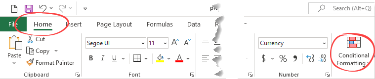
2. Select the Home tab, and locate the Styles Group. Click Conditional Formatting.
3. Locate the Color Scales drop-down menu.
Pick the preferred color scheme and click it.
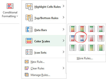
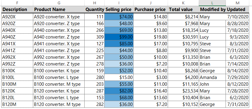
Use the red-white-blue color scale.
The range shows the prices by color. Red cells are higher values, white is the median, and blue cells have lower values.
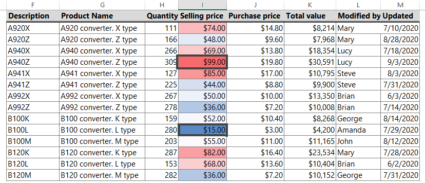
Explanation: By default, Excel calculates the median and applies three colors to highlight cells.
To calculate the median, use the formula below:
=MEDIAN(I2:I15) = $53.50
- Cell I5 holds the maximum value ($99), which is red in this case.
- In cell I11, you can find the minimum value ($15) with blue.
- All other cells are colored proportionally.
Example
Select the range I2:I15 to change the default rule.
To do that, click Conditional Formatting and select the Manage Rules command from the drop-down list.
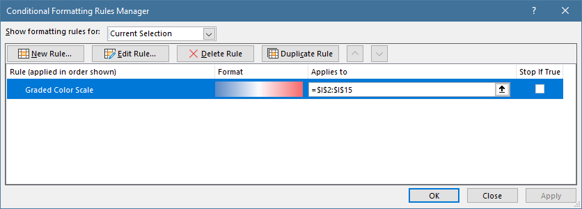
After clicking Manage rules, the Edit Formatting Rule window will appear.
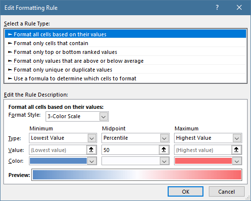
Click ‘Edit Rule.’
If you want to modify the default settings, you can do that (for example, change the formatting style, apply new scales or change the limits for the minimum and maximum range.
Tip: you can use a shortcut to reach this window by clicking More Rules.
To apply a simple color scale without showing the mid-range values (apply only two colors), do the following:
On the ‘Edit the Rule Description’ tab, change the formatting style to ‘2-Color Scale.’
Select the color picker (use the drop-down list), add white fill for the minimum value, and use blue for the maximum value.
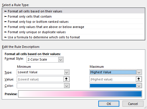
Click OK, then ‘Apply’ to check the result:
Additional training materials: