Learn how to use multiple conditions and formulas in conditional formatting to apply multiple criteria (AND, OR, LEFT, RIGHT) to a single cell or a range.
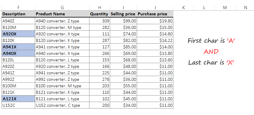
Now let’s talk about the logical functions. In this section, we’ll show you how to create effective formulas to build a complex rule. First, we will create a new rule to highlight any cell in the Description column that starts AND ends with the given characters.
How to create multiple conditions in Excel
To highlight cells in line with multiple conditions, follow the steps below:
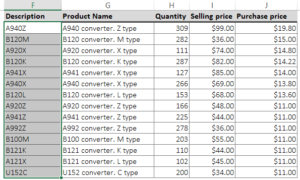
1. Select the range to apply formatting rules
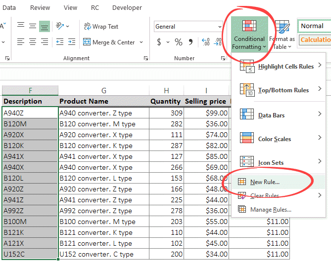
2. Click Home > Conditional Formatting > New Rule.
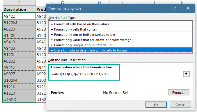
3. Choose ‘Use a formula to determine which cells to format‘, and type the formula: =AND(LEFT(F2,1)=” A”, RIGHT(F2,1)=” X”). We want to search cells in the Description column for an ‘F’ and highlight that cell when multiple conditions are true. To do this, we’ll use Excel’s LEFT and RIGHT formulas, with the AND formula, to lookup the A and X values.
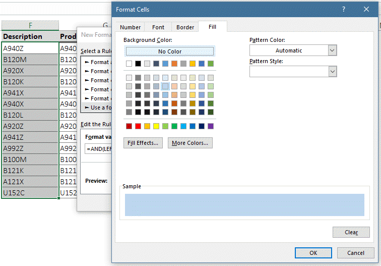
4. Click on the Format button and add your preferred style
5. Click OK twice to return to the Conditional Formatting Rules Manager window.
6. Use the formatting to the selected range by clicking ‘Apply‘ and then click Close.
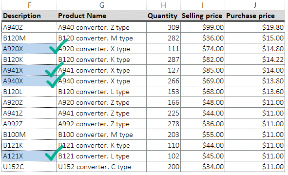
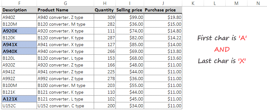
Your spreadsheet will focus on all cells in Description that meet ALL conditions. Excel will reflect every cell in the range selected with the first character = A, AND the last character = X by changing the background color.
Explanation
We use AND at the beginning of the formula to apply multiple conditions at the same time.
Apply the LEFT function when you want to extract a given number of characters starting on the left side of the text. For example, LEFT(“A920X”,1) returns “A.”
Use the RIGHT function to extract characters starting at the right side of the text. The Excel RIGHT function extracts a given number of characters from the end of a string.
For example, RIGHT(“A920X”,” 1) returns “X.” So, this example is just one of the hundreds of different formulas you could enter with the AND function.
Tip: If you want to use multiple rules instead of multiple conditions, you can do it without trouble. Learn how to create a rule that depends on another cell.