Learn how to use conditional formatting based on another cell and create a rule that depends on another cell value in Excel.
Conditional formatting enables us to determine highlights based on the value of a referred cell. In the referred cell, we can modify the values arbitrarily. If the value changes, then the highlight of the given range (icons, shapes, custom formatting, etc.) will dynamically change also.
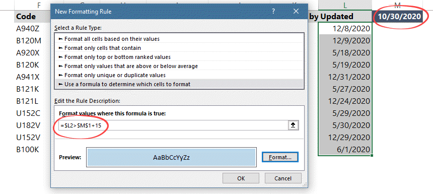
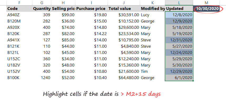
In the example, you want to highlight all the dates in column N when they are more than 15 days newer than the date I enter in cell M2. Select the Updated column (range N2:N24) in the sample file.
Steps to use conditional formatting based on another cell
- Click Conditional Formatting on the Home tab of the ribbon
- Click New Rule. A popup window will appear.
- Choose ‘Use a formula to determine which cells to format’.
- Enter the formula =$M2>$N$1+15
- Click the Format button and select your formatting style.
- Click OK.
Explanation:
In this expression, Excel evaluates values in column ‘M.’ M2 reference the first cell in the selected range. You can apply this conditional formatting rule for this range. Use the ‘$’ symbol for M2. Press F4 twice ($N$1) to apply absolute reference because N1 is an absolute value. The conditional formatting rule always uses this cell. What’s the meaning of the second part of this formula ‘>$N$1+15’? Every cell that is more than 15 days after the date in cell N1 is appropriate to our criteria!
Result: Excel will highlight cells where the difference between dates is more than 15 days.
How do I change conditional formatting based on another cell?
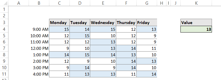
To highlight cells based on a value in another cell, use this conditional formatting formula to the range C4:G11 is: =C4>=$K$4. Thus, in this example, you want to highlight cells in the range C4:G11 when they are greater than the value entered in cell K4.
How do you conditional format a column based on another column?
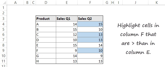
To use conditional formatting based on a value in another column, create a rule using a formula for range D5:D14: =$F4>$E4.
Excel highlights values in column F that are greater than in column E.