
Use a few steps to learn how to change shape color based on cell value in Excel. Get the VBA example or use conditional formatting!
This tutorial will explain how to create interactive charts using conditional formatting. Believe it or not, changing chart objects’ shape color is possible using VBA tricks! Then, you will learn how to extend the formatting cells function and move to the next level in Excel.
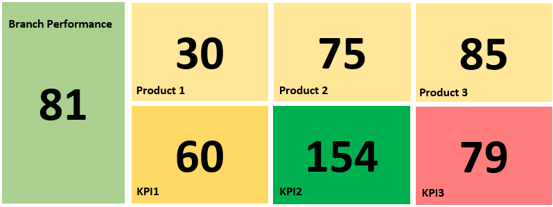
Here is a grid layout example below. We love it! If you read the article, you can create advanced report elements.
In the next section, we’ll introduce the manual way. Preparing the code is a bit time-consuming, but we’ll help you!
Change Shape Color using conditional formatting
Dynamic shapes play an important role and show your data in Excel creatively. Lastly, it is a great addition to any dynamic chart.
Worksheet Events – Using triggers in Excel
What is the Worksheet Event? Excel can automatically run any macro when data in any cell on the Worksheet changes. Therefore, we can run our code only when specific cells change. We’ll use this method to create dynamic widgets based on a cell’s value.
Our goal is to create formatted color shapes based on cell value. For example, we are trying to conditionally format shapes in Excel to red, yellow, or green based on a cell instruction stating ‘red,’ ‘yellow,’ or ‘green.’ We’ll give you a complete solution using simple VBA macros.
Steps to create conditional logic for shapes
- Open the VBA editor. Because we don’t want manually to run any code, Select Sheet1 and place the code below:
Private Sub Worksheet_Change(ByVal Target As Range)
If Range("B3") = "red" Then
ActiveSheet.Shapes.Range(Array("Shape1")).Select
Selection.ShapeRange.Fill.ForeColor.RGB = RGB(255, 0, 0)
Else
If Range("B3") = "yellow" Then
ActiveSheet.Shapes.Range(Array("Shape1")).Select
Selection.ShapeRange.Fill.ForeColor.ObjectThemeColor = msoThemeColorAccent4
Else
If Range("B3") = "green" Then
ActiveSheet.Shapes.Range(Array("Shape1")).Select
Selection.ShapeRange.Fill.ForeColor.ObjectThemeColor = msoThemeColorAccent6
End If
End If
End If
ActiveSheet.Cells(3, 2).Select
End Sub
Take a closer look at the macro! We’ll test more than one condition. In this example, it’s necessary to use multiple IF statements in one subroutine.
If the value (text) on the given cell = “red,” then the code applies a red fill on the ‘Shape1’. If the cell is empty or the text is not equal to “red,” the macro jumps into the next case.
To build up a macro that reflects this logic, we can start by testing to see if the cell value is equal to ‘Yellow.’ If the result is TRUE, we shade the vector object as yellow. If the condition is FALSE, we move forward and check the result of the third IF function.
Finally, we test whether the cell value equals “green.” If TRUE, we return the object, and it will be green. If FALSE, we exit the subroutine.
Now save the Workbook in an ‘xlsm’ format.
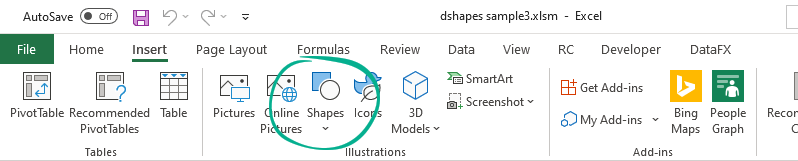
2. Create a new sheet and insert a new object. On the ribbon, select the Insert menu, then choose Shapes.
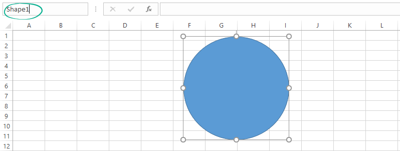
3. Rename the default name to ‘Shape1’.
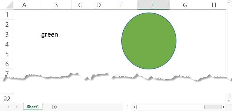
4. Let’s check the macro! Enter the text “green” in cell B3. Now, the macro will apply a green color.
Work without limits in Excel: Dynamic colored shapes
When using Excel to create reports, there is a limitation to what you can do using only the cells available. So, how do we transform our presentation to develop interactive, value, and color-based widgets?
This section reveals my best tricks for building interactive dynamic shapes containing conditional formatting rules. In addition, you can learn something unique about this topic.
Check the result before we get into the middle of the guide: The shape’s colors depend on the cell value, and it will change dynamically!
So follow these steps below to change the shape color:
- First, choose an object from the list and insert a new object.
- Use the Name Box to change the name from the default to “Shape1”.
- It’s important to use specific names for every object to identify the vector objects easily.
- Check the first row on the setup Worksheet; now, we’ll explain how this parameter table works:
The shape is:
- Green, if the actual value is greater than the upper limit,
- Yellow, if the actual value is between the upper and lower limit,
- Red if the actual value is less than the lower limit.
Color1, Color2, and Color3 represent the color scale. Change the color scheme if you prefer a custom color theme.
Link the object to the value
If you want to link the object to a value in a cell, make sure the shape is selected from its edges.
Explanation: If the cursor is not blinking inside the shape, you assign the value. Click the formula bar, press “=”, and select the cell with the value you want to point to. In this case, cell H2.
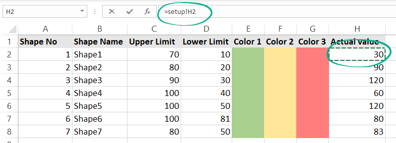
The cell value will be assigned to the given object. In this case, the current value is 70. The value is between the upper and lower range so that the shape color will be yellow.
Format the value, increase the font size, and align the text. Because we use triggers, you can modify the actual value; the dynamic shape will reflect the changes.
Need more widgets to create a stunning report? No problem! Insert a new row and fill in the necessary information for the new vector object.
Conclusion: Change the Shape Color and boost your report!
Using conditional formatting and shapes for stylish Excel reports is a bright idea. Use our free templates to show how your KPIs perform based on your targets. VBA is a perfect tool for developing suitable solutions in Excel.
Okay, it’s time to play with the template. Download the practice file. Take a closer look at the VBA section and create your solution.
Additional resources: