Learn how to use XLOOKUP with multiple criteria by concatenating lookup values and lookup arrays inside the formula.
XLOOKUP multiple criteria: The Basics
In Excel, you can modify the XLOOKUP formula to work with multiple criteria in a few ways. By default, XLOOKUP is for a single lookup value. However, you can join multiple criteria to build a single lookup value or use arrays. For example, if you have multiple employees with the same name but in different departments or years, you must use more than one criterion to get the correct data. XLOOKUP can handle these cases using multiple conditions for a fast lookup.
How to build the Lookup values for multiple criteria
Take a look at the example below! We will use the basic syntax of the function and use only the required arguments:
=XLOOKUP(lookup value, lookup array, return array)
Because we want to use multiple criteria, we concatenate the arguments.
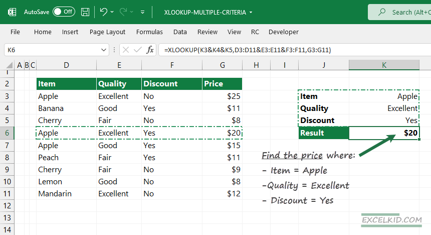
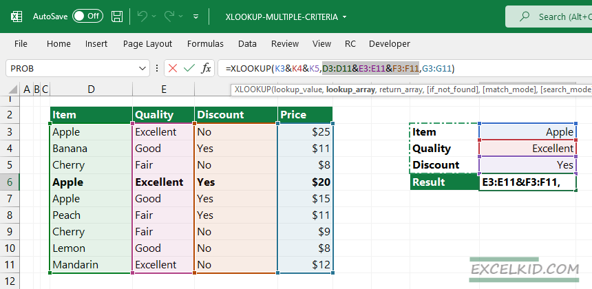
=XLOOKUP(K3&K4&K5, D3:D11&E3:E11&F3:F11, G3:G11) =$20
In the example, our goal is to find the item’s price, where the item is apple, the quality is excellent, and the price is discounted.
Using VLOOKUP, we can’t use arrays inside the formula. With XLOOKUP, we’ll construct arrays in the formula using them as arguments.
=XLOOKUP(value1&value2&value3, range1&range2&range3, results)
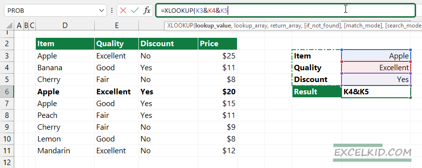
Construct the lookup_value (the first argument of the XLOOKUP function) using the “&” sign to create a single argument from the multiple criteria.
Let us see the arguments that contain multiple criteria:
- lookup value: K3&K4&K5
- lookup_array: D3:D11&E3:E11&F3:F11
- return_array: G3:G11
In the example, the formula in K6:
=XLOOKUP(K3&K4&K5, D3:D11&E3:E11&F3:F11, G3:G11) = $20
XLOOKUP returns $20, the price for a discounted but excellent quality apple.
Note: In the case of multiple criteria, Excel evaluates the formula using the following logic:
- lookup_value: “AppleExcellentYes“
Tip: If you are working with Microsoft 365 or Excel 2021, you have dynamic arrays, and you do not need to use Ctrl+Shift+Enter. However, for older versions, you might need to confirm the formula with Ctrl+Shift+Enter to create an array.
If you want to look at the demonstrated example, download the practice file!