Learn how to use XLOOKUP to match text values with the help of the 5th argument, wildcard character match mode.
How to lookup matching text values
One of the powerful features of the XLOOKUP function is the native wildcards support. You enable wildcards, locate the 5th argument (match mode), and set the parameter to 2.
General formula:
=XLOOKUP(“*”&lookup_value&”*”,lookup_array, return_array,if_not_found,2)
First, we use named ranges to simplify the formula:
- ID = range C3:C8
- Price = range D3:D8
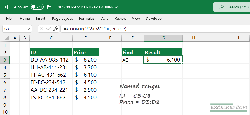
Take a closer look at the formula in cell G3:
=XLOOKUP(“*”&F3&”*”,ID,Price,”value not found”,2)
- lookup value – F3
- lookup array – ID is a named range, C3:C8
- return array – Price is a named range, D3:D8
- if not found – the value in case of no match found, “value not found.”
- match mode – to switch wildcard match mode on, use 2
In the example, we leave the 6th argument (Search mode) by default – first to last.
Evaluate the match text lookup formula
The first thing that you keep in mind: you have to concatenate the lookup values with two wildcards (*).
Use the “&” character to join values “on the fly”. Here is the method to merge the lookup value:
Lookup value: “*” & F3 & “*”
Now the formula looks like the below:
=XLOOKUP(“*AC*”, ID, Price, “value not found”, 2)
This part of the formula tries to find the first matching text that contains the lookup value. For example, the first match that contains the “AC” string is “TT-AC-431-662” located in the third row of the table. In case of a match -like in the example – the function returns with the price in the same row, $6100.
Workaround with VLOOKUP and text contains lookups
If you are not using the latest Microsoft Excel, no problem. There is a workaround with the good old VLOOKUP function.
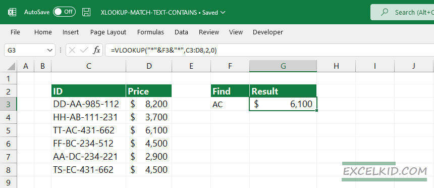
Here is the solution for VLOOKUP:
=VLOOKUP(“*”&F3&”*”,C3:D8,2,0)
Explanation:
Concatenate the lookup value with an asterisk (*). The formula searches the lookup value in range C3:D8. Press Enter, then the formula returns the corresponding value from the second column; the result is $6100.
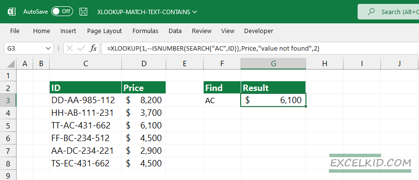
Lookup text contains using XLOOKUP & SEARCH
There is a further alternative of lookups for “text contains” or partial match cases. If you work with the SEARCH function and FIND function in the same XLOOKUP formula, you’ll get the correct result.
The non-case-sensitive formula example:
=XLOOKUP(1,–ISNUMBER(SEARCH(“AC”,ID)),Price,”value not found”,2)
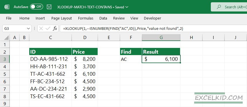
XLOOKUP & FIND (case-sensitive match)
If you are looking up a case-sensitive match, replace the SEARCH function with the FIND function.
Formula:
=XLOOKUP(1,–ISNUMBER(FIND(“AC”,ID)),Price,”value not found”,2)
The last two formula uses boolean logic; read more about it.