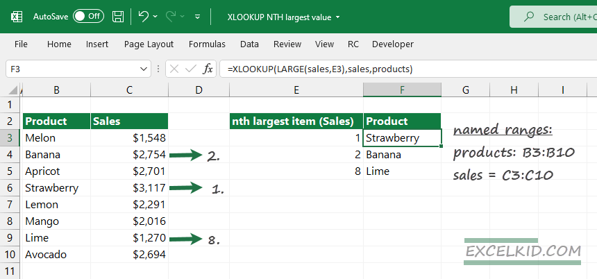
To get the name of the nth largest value in a range, use the XLOOKUP functions with the LARGE function together.
In the example, we will use the LARGE function to calculate the lookup value for the formula based on the XLOOKUP function.
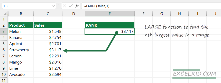
The LARGE function uses simple logic to find the nth largest value in a range. For example, to extract the largest value from the range C3:C10, use the formula:
=LARGE(sales, 1), where ‘sales’ is a named range.
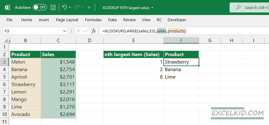
XLOOKUP get the name of the nth largest value
In the example, we want to find the largest value in a range, so the function returns $3117. In other words, we now have the XLOOKUP function’s first argument.
Let’s configure the arguments:
- lookup_value: =LARGE(sales,1)
- lookup_array is named range, ‘sales‘ (C3:C10)
- return_array is a named range, ‘products’ (B3:B10)
We are not using the optional arguments to find the nth largest value in this case. Instead, XLOOKUP will perform the lookup based on the LARGE(sales,1) expression and check the range C3:C10. If the function finds a match, return the name of the corresponding item.
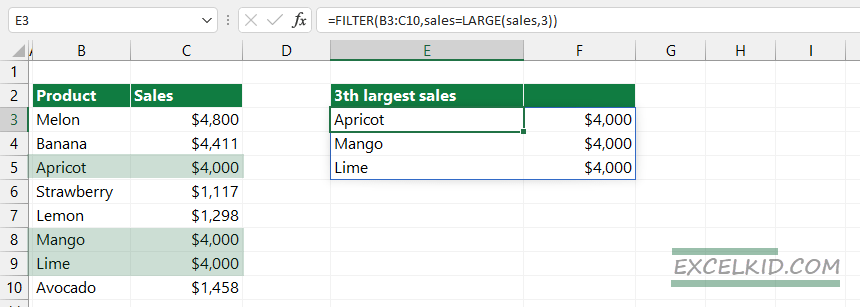
Workaround with multiple matches (duplicated values)
What if we have multiple matches? In the following example, we want to find the third-largest value in a range. The nth largest values may be the same in Excel, and the LARGE will return multiple matches.
Take a closer look at the picture below:
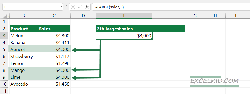
Use the FILTER function to extract all records that meet the criteria.
=FILTER(B3:C10,sales=LARGE(sales,3)