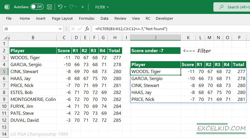
The Excel FILTER function filters range with given criteria and extracts matching records from an array of filtered values.
FILTER is one of the dynamic array functions available in Microsoft 365.
Syntax and Arguments
Syntax:
=FILTER(array, include, [if_empty])
Arguments:
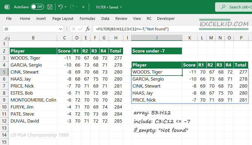
- array: the range or array that contains the data for the filter
- include: the criteria array
- if_empty: optional argument for error-handling, in case of no result
How to use the FILTER function
Using the FILTER function, you can extract a range of data based on the given criteria. Then, when evaluating the formula, the result is not a single value. Instead, you will get an array of matching values from the source range as a result.
In other words, the FILTER function extracts the matching records from a list or table and uses one or more logical tests. A great advantage is that you can include the logical test in the function argument. As a result, FILTER simplifies tasks in Excel. For example, it can look up data based on score, names, category, or anything else.
The FILTER function uses three arguments: two required and one optional. The array and include arguments are required. The if_empty argument is optional.
- The first argument, the ‘array’, is the range you want to filter.
- The ‘include’ argument may contain one or more logical tests. The result is always TRUE or FALSE, which follows the boolean logic.
- The third argument, ‘if_empty’, is error-handling when the FILTER functions do not find matching records. Therefore, using other error-handling functions like IFERROR or IFNA is unnecessary.
In practice, the third argument is a text string like “Not found” or “No matching records found”. If you want to show a “blank” cell in case of no matching records, use an “empty string”.
The result is a dynamic array, and here are further advantages of using the FILTER function. If you change the source range structure by deleting rows or columns, the results table, Excel will update the result automatically. You can resize the source range, too, without any trouble. FILTER spills the return array into multiple cells.
Filter Function Examples
We have learned the basics; let us see some practical examples.
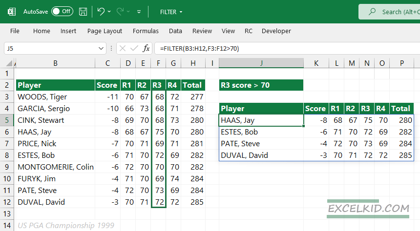
Filter function: Basic usage
In the example, we want to extract the matching records greater than 70 in column F and use only the first two required arguments.
=FILTER(B3:H12, F3:F12>70)
The formula will extract the corresponding rows into a multi-column array. The destination range is J5:P8.
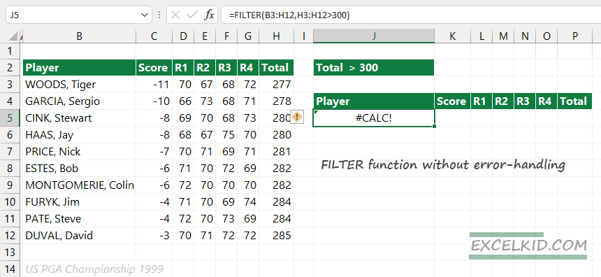
Error handling in case of no matching data
The FILTER function may return without any match. Using the third (if_empty) argument, you can manage the case if no matching data is found. For example, let us suppose that we want to filter data in the Total column. First, find the matching records where H3:H12 > 300.
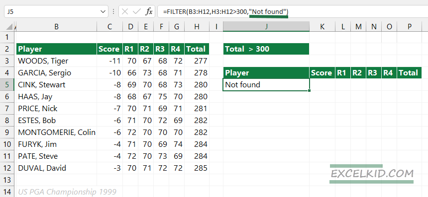
Using only two arguments, you will get a #CALC! error:
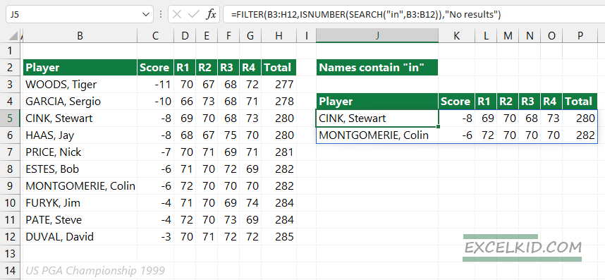
Filter values that contain text
In the following example, we want to filter specific records that contain specific text using a logical test. For simplicity, extract the records where the player’s name contains the “in” text!
Generic formula:
=FILTER(range1, ISNUMBER(SEARCH(“text_to_find”, range2)))
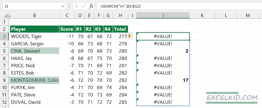
Evaluate the formula from the inside out:
The SEARCH function finds the text “rd” inside the player’s data in B3:B12. Our list contains ten records, and the result array will be the same size.
=SEARCH(“in”, B3:B12))
A result is a number if the text is found; otherwise, the array contains a #VALUE error.
=ISNUMBER(SEARCH(“in”, B3:B12))
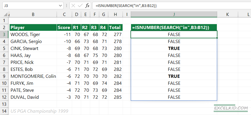
This array provides the input for the FILTER function. FILTER will extract the records where the result is TRUE.
Finally, we will use the “Not found” text string in case of no matching data.
=FILTER(B3:H12, ISNUMBER(SEARCH(“in”, B3:B12)), “no results”)
Filter by date
Using the example mentioned above, you can filter records based on date criteria. In the example, we want to extract the records where the date of birth is greater than 1970.
Formula:
=FILTER(B3:D12, YEAR(C3:C12)>1970)
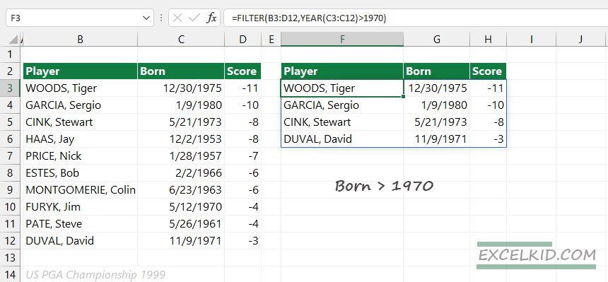
The YEAR function returns an array that contains the following values:
{1975, 1980, 1973, 1953, 1957, 1966, 1963, 1970, 1961, 1971}
The logical test will compare the array items to 1970 using the “greater than” logical operator. If the result is TRUE, the FILTER function will extract the given record.
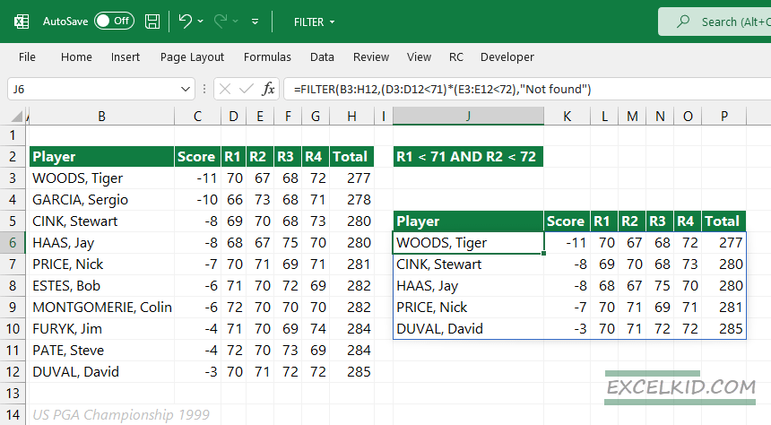
Filter based on multiple criteria
The included argument is flexible, and you can use multiple criteria
For example, you want to filter records where the Round 1 score is less than 71 and the Round 2 score is less than 72.
Formula:
=FILTER(B3:H12, (D3:D12<71)*(E3:E12<72), “Not found”)
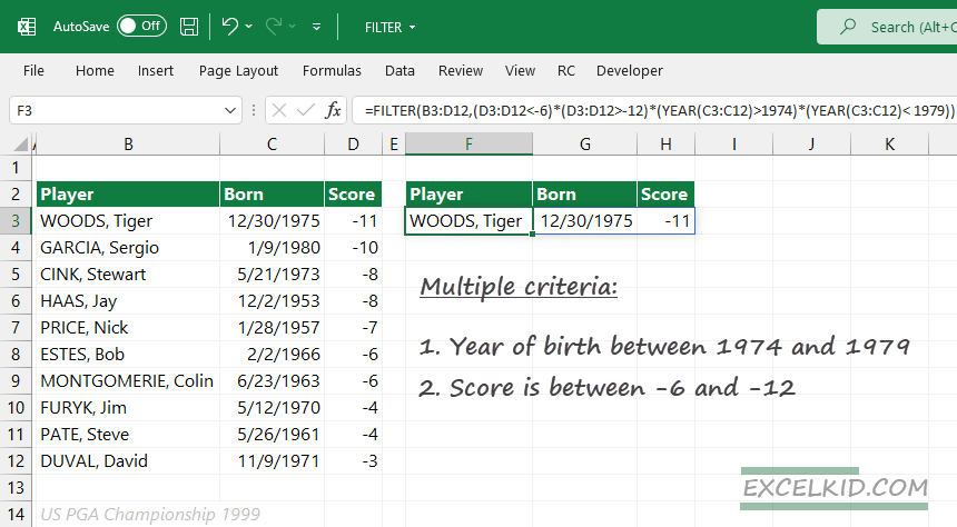
Filter function and complex scenarios
For example, the generic formula below filters based on four different conditions:
- year of birth between 1974 and 1979
- the final score is between -6 and -12
The FILTER function can handle advanced filtering scenarios through logical expressions.
Formula:
=FILTER(B3:D12, (D3:D12<-6)*(D3:D12>-12)*(YEAR(C3:C12)>1974)*(YEAR(C3:C12)< 1979))
The Excel FILTER function is great. Download the practice file and play with it!
Additional resources