To sum multiple rows or columns based on a lookup value, you can use the SUM function with the XLOOKUP function.
Even if we have a definitive XLOOKUP guide, we learn something special daily. Today’s example will be on how to find the matching value in a table and sum multiple rows or columns. The method we demonstrate completely replaces the recent VLOOKUP and HLOOKUP functions.
How to SUM multiple rows values based on a lookup value
This solution provides a powerful VLOOKUP alternative. Use a vertical lookup to find the matching value and sum multiple columns in the same row.
For the sake of simplicity, we will use named ranges:
- Products = B3:B9
- Data = C3:E9
Configure the XLOOKUP function arguments:
- lookup_value: G3
- lookup_array: “products”
- return_array: “data”
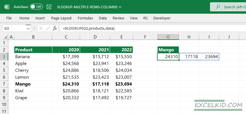
Formula:
=XLOOKUP(G2, products, data)The result is a dynamic array that contains three numeric values.
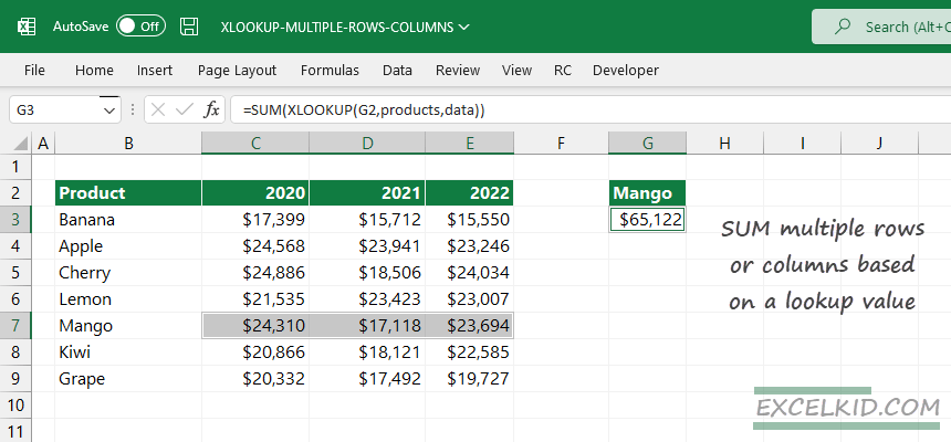
Because we want to get the result as a single value instead of an array, we use the SUM function to compile the array into one cell.
Formula:
=SUM(XLOOKUP(G2, products, data))Steps to SUM multiple column values based on a lookup value
The following example is based on a horizontal lookup and replaces the HLOOKUP function. First, create a horizontal lookup formula to find the matching value and sum multiple rows in the same column.
Our goal is to find the sales in 2022; In this case, we want to find the matching value in the header section.
Create a new named range; “year” will refer to range C2:E2.
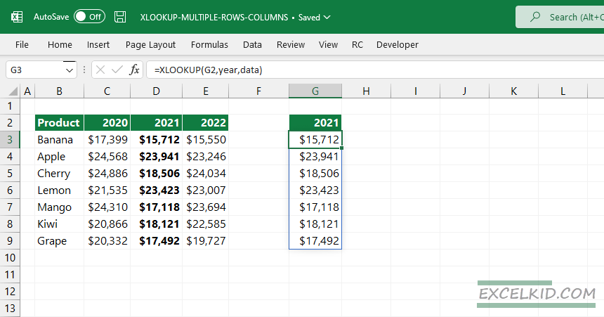
Formula:
=XLOOKUP(G2, year, data)The formula will search the lookup value in the header and return the entire column values in case of a match. As we stated before, the result is an array containing all values we want to sum. We want to return the sum, so combine the XLOOKUP function with the SUM function.
Formula:
=SUM(XLOOKUP(G2, year, data))The result is a single value.