To find the first or last positive value in a list (row or column), use the XLOOKUP, SIGN, INDEX, or MATCH functions.
Generic Formula to lookup the first positive value
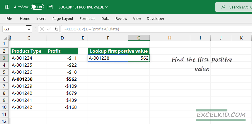
XLOOKUP simplifies everything so that we will use it as default. To find the first positive value in a range, use this formula where “rng” is the range of cells where we try to find the matching value:
=XLOOKUP(1,--(rng > 0), rng)Based on the generic formula above, enter the cell F4:
=XLOOKUP(1,--(profit>0), data)As usual, it is worth using named ranges; “profit” refers to range D3:D10, and “data” refers to B3:C10.
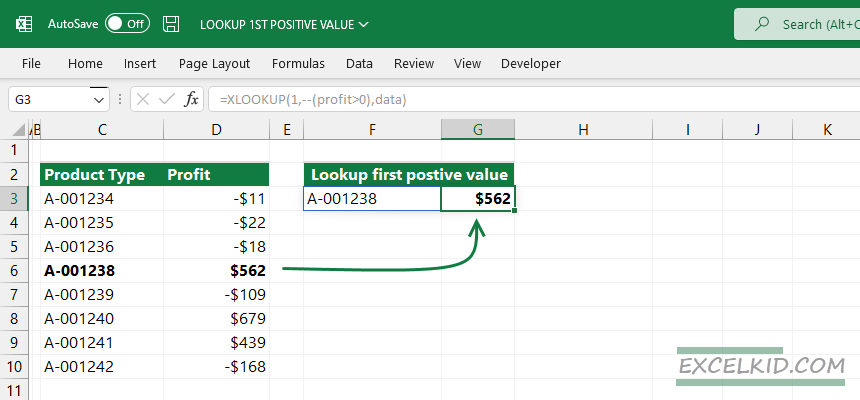
The result is the 4th row in the range since this is the first positive number in the Profit column. The XLOOKUP-based formula will return an array that contains the result and the corresponding ID.
How to find the first positive value
All examples use the same logic: lookup the first positive value in a range on different Excel versions.
XLOOKUP and SIGN functions
First, let us see the way to find the first positive value using the SIGN and XLOOKUP functions. The SIGN function returns the sign of a number. So, use “1” as an argument. Note: if you find negative values or zeros, use the -1 or 0 arguments; the method is the same.
The point is that you can use the output of the SIGN functions as a lookup value! Enter the following formula in cell F3:
=XLOOKUP(1,SIGN(profit), data)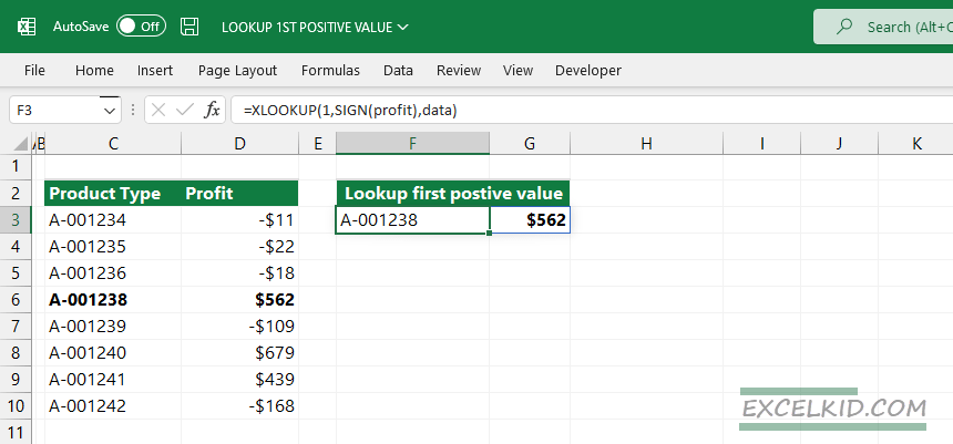
Lookup the last positive value in a list
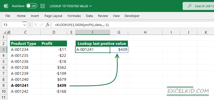
If you want to find the last positive number, add extra parameters to the XLOOKUP function. Apply the 6th argument to control the search mode.
Formula:
=XLOOKUP(1,SIGN(profit),data,,,-1)Result:
INDEX and MATCH to get the first positive value
If you are not using a Microsoft 365 subscription, there is an alternative way to get the same result as the example above. The following INDEX and MATCH combination works fine with Excel 2013, Excel 2016, or Excel 2019.
Here is the formula to lookup the first positive value in a range using INDEX + MATCH:
=INDEX(data,MATCH(1,--(profit>0)),0)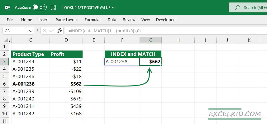
Evaluate the formula from the inside out! The “–(profit>0)” part will convert boolean values (TRUE or FALSE) to 0 and 1.
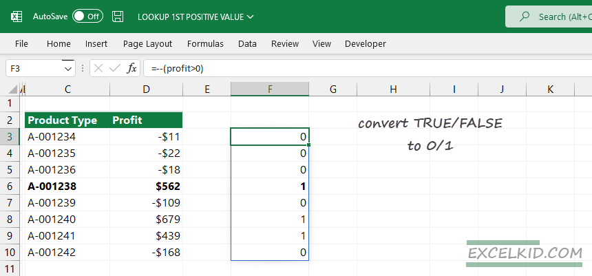
Apply the MATCH function to extract the position of the first positive value from the lookup array. The result array looks like this:
={0, 0, 0, 1, 0, 1, 1, 0}We find the positions where the cell value = 1. So, the array contains three values that are greater than 0. The following formula will get the first position where the profit > 0. It is the 4th row in the table.
=MATCH(1,--(profit>0),0) = 4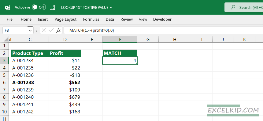
The INDEX function uses the result as a row_num argument:
=INDEX(data,MATCH(1,--(profit>0)),0)Find the last positive value using the LOOKUP function
The LOOKUP function searches for a value from a one-row, one-column range, or array.
Configure the function arguments like this:
- lookup value = 2
- lookup vector = 1/(profit>0)
- result vector = profit
Formula:
=LOOKUP(2,1/(profit>0),profit)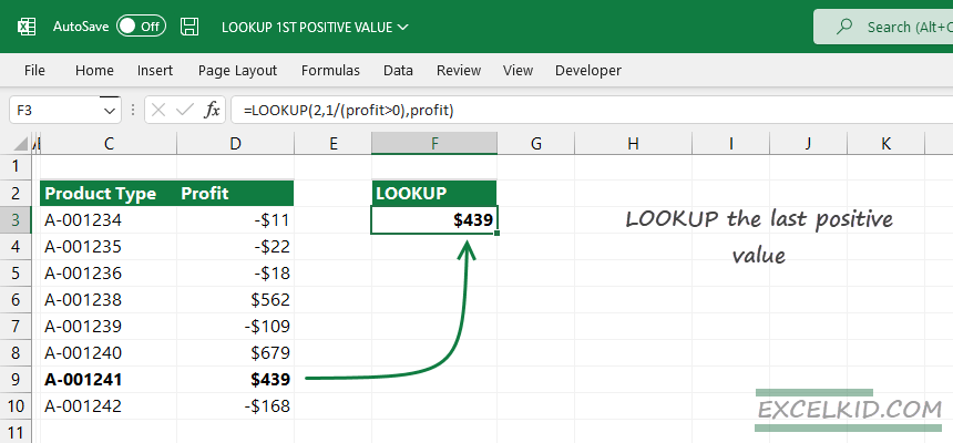
Note: the result vector is an optional argument.
Lookup first positive value using INDEX and FILTER functions
The following example will list all matching values using the INDEX and FILTER functions. The result array contains two rows; the result includes all columns in the source table.
FILTER function arguments:
- array: data
- include: profit > 0
Formula:
=FILTER(data, profit>0)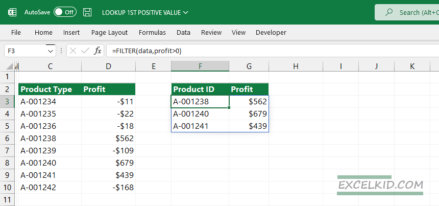
The result contains all records where the profit > 0, so we get all cells with positive values. Therefore, we have three records, but we need to use only the last one to get the last positive value in the array.
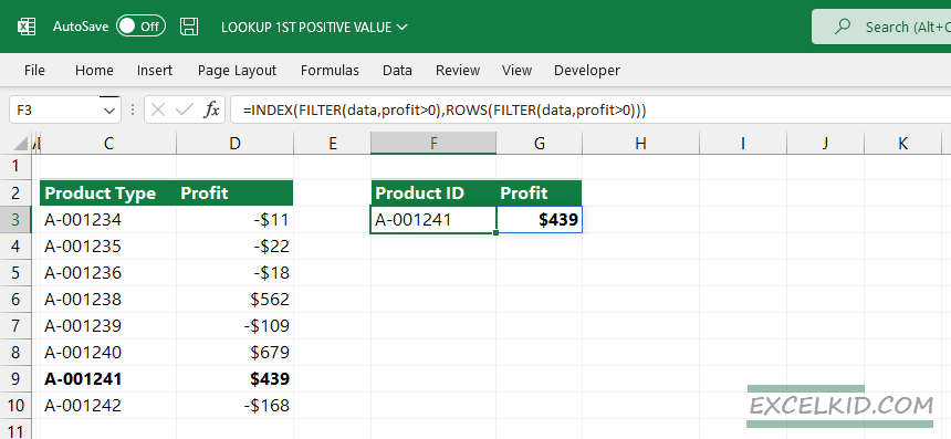
The ROWS function will get the position of the last positive item in the array. Finally, the INDEX function will use the position as an argument to get the proper result:
=INDEX(FILTER(data,profit>0),ROWS(FILTER(data,profit>0)))