Learn how to lookup the first negative value in a range using the XLOOKUP function or INDEX and MATCH functions.
Generic Formula
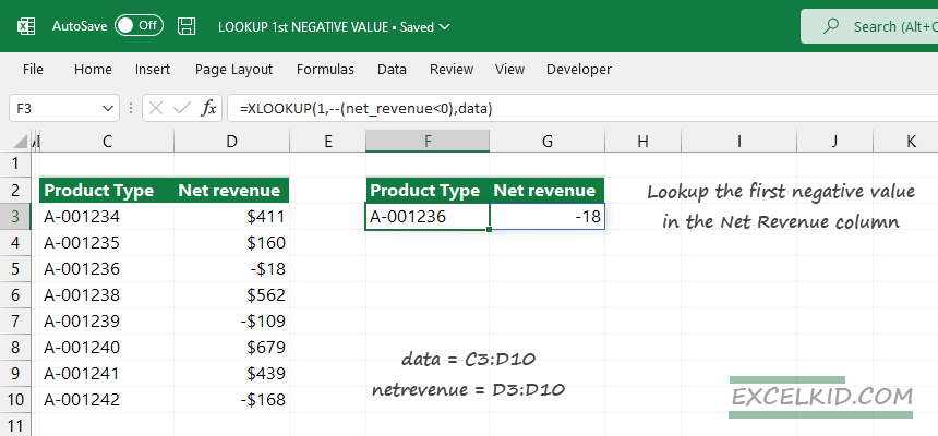
Here is the generic formula to lookup the first negative value in a range:
=XLOOKUP(1,--(rng < 0), rng)In the formula, “rng” is the range where we find the first negative value; enter the formula in cell F3:
=XLOOKUP(1,--(net_revenue<0),data)In the example, net_revenue and data are named ranges and refer to C3:C10 and B3:C10.
The result is the 3rd row in the range since this is the first negative value in the Net Revenue column. The formula returns an array and will also contain the matching value and the corresponding Product type.
In the following chapters, we’ll show some alternative methods if you do not have built-in XLOOKUP support available.
Formulas to lookup first negative value
The following 4 examples use the same logic; that is the following: lookup the first negative value in a range on different Excel versions.
SIGN function
First, let us see the most elegant way to lookup the first negative value. The SIGN function returns the sign of a number. If the number is positive, the function returns with 1, zero if the number is zero, and -1 if the number is negative.
Use the SIGN functions result as a lookup value to find the first negative item in the Net revenue column:
Enter the following formula in cell F3:
=XLOOKUP(-1,SIGN(net_revenue),data)
XLOOKUP and double negative
If you have a Microsoft Excel subscription, the fastest way is to use the XLOOKUP function and keep in mind the boolean logic.
Because our lookup value is numeric (1) and the result array contains booleans, we have to convert the array from TRUE/FALSE to 1 and 0. To convert booleans (true and false) to numeric values (1 or 0), use the double negative method (–).
Formula:
=XLOOKUP(1,--(net_revenue<0),data)As usual, we will evaluate the most advanced formulas from the inside out. Therefore, we strongly recommend you use this step-by-step method.
First, enter the formula in cell F3:
=net_revenue<0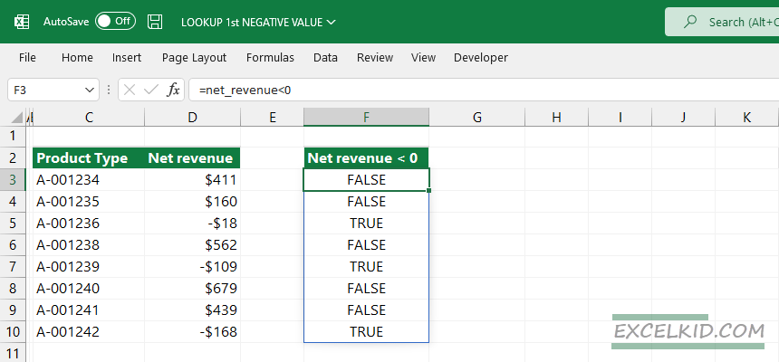
In the example, there are 8 values in the Net Revenue column; the formula will return an array that contains booleans, TRUE, and FALSE values.
{FALSE, FALSE, TRUE, FALSE, TRUE, FALSE, FALSE, TRUE}The problem is that our primary goal is to use 1 (numeric value) as a lookup value. Because our lookup value is numeric (1) and the result array contains booleans, we have to convert the array from TRUE/FALSE to 1 and 0. To convert booleans (true and false) to numeric values (1 or 0), use the double negative method (–).
To convert the boolean array to a numeric array, use the formula below:
=--(net_revenue<0)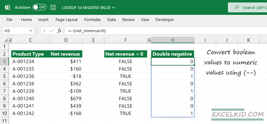
As a result of the formula, we now have an array that contains numeric values:
{0,0,1,0,1,0,0,1}To find the first negative value in a range, we must find the first TRUE value (=1).
Configure the XLOOKUP function:
- lookup value = 1
- lookup array = {0,0,1,0,1,0,0,1} = –(net_revenue<0)
- return array = data (C3:D10)
=XLOOKUP(1, --(net_revenue<0), data)If you do not use the 5th argument of XLOOKUP (match mode), the function will use an exact match by default. The formula finds the first 1 in the Net Revenue column, returns row 3 from the data table, and spills the matching values (Product type and Net Revenue) into cells F3 and G3.
Workaround with INDEX and MATCH functions
Let us see the possible workaround for using Excel 2016 or Excel 2019. First, use the INDEX and MATCH combinations to find the first negative value in a range.
Formula to lookup the first negative value in a range using INDEX + MATCH:
=INDEX(data, MATCH(1,--(net_revenue<0),0),0)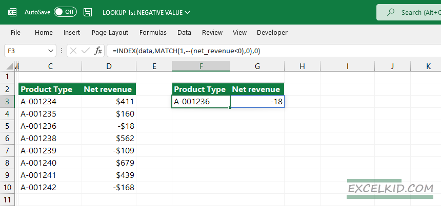
Evaluate the following part of the formula:
The –(net_revenue<0) expression will convert the boolean values to 1 and 0.
=MATCH(1,{0;0;1;0;1;0;0;1;},0),0)After that, the MATCH function gets the lookup value (1) position in the lookup array (3).
=MATCH(1,--(net_revenue<0),0) = 3Set the INDEX functions’ column_index argument to 0 so the function will return the Product Type and Net Revenue columns. INDEX will use the result as a row_num argument:
=INDEX(data,3,0)Note: In the example, we use the latest Microsoft 365 for Excel, so it is not necessary to use brackets and the Ctrl + Shift + Enter keys. However, if you are working with a previous Excel version, you have to use Ctrl + Shift + Enter like the example below:
={INDEX(data,MATCH(1,--(net_revenue<0),0),0)}Lookup negative values using the FILTER function
First, use the following formula to list all matching values using the INDEX and FILTER functions. It is good to know that if you want to return all negative values, use the FILTER function standalone. The result array contains three rows; the result includes all columns in the source table.
Configure the FILTER function:
- array: data
- include: net_revenue<0
Formula:
=FILTER(data,net_revenue<0)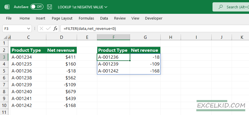
The returned array contains three records, and INDEX will be used as the array argument. Set the second argument of the INDEX function to 1. To find and list only the first negative value in an array, append the formula with the INDEX function:
=INDEX(FILTER(data,net_revenue<0),1)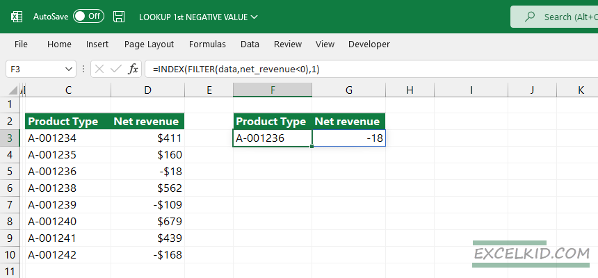
The final result is -18, the first negative value in the given range.