Learn how to use the XLOOKUP function with Boolean expression (OR logic). To do that, set the lookup value to 1.
XLOOKUP is our favorite dynamic array function, which you can use in various situations.
Generic formula to use a boolean or logic
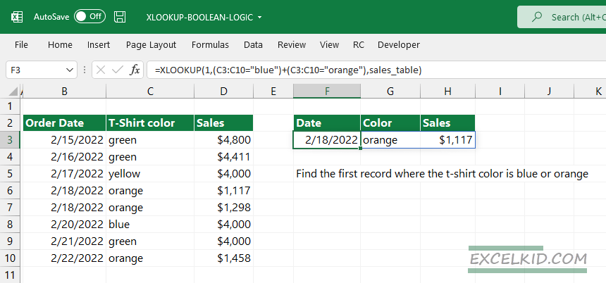
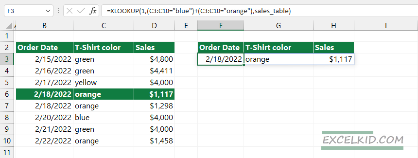
In the example, our goal is to find and list all records where the color is “orange” or “blue”.
Formula:
=XLOOKUP(1 ,boolean_expression, data)
The arguments of the XLOOKUP function:
- lookup value is 1; in other words, TRUE.
- lookup_array is an expression, and it has two possible outputs (TRUE or FALSE) based on the boolean logic
- the lookup array is named range, “sales_table”, (B3:D10)
Note: sales_data is a named range and is referred to as range B3:D10.
Formula:
=XLOOKUP(1, (C3:C10=”blue”)+(C3:C10=”orange”), sales_data)
Good to know when you use boolean logic; Excel follows the rules below:
- Multiplication (*) corresponds to the AND operator
- Addition (+) corresponds to OR operator
XLOOKUP with Boolean OR logic
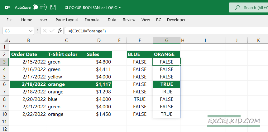
Working from the inside out, we will evaluate the following expressions:
=C3:C10 = “blue”
=C3:C10 = “orange”
Take a look at the first array in column F. If the color is “blue” in the given row in range C3:C10, the expression returns with TRUE (1), else FALSE (0).
The =C3:C10 = “orange” expression gets TRUE (1) if the cell value is “orange”, else gets FALSE (0).
We will apply math operators to convert the TRUE and FALSE outputs to 1 or 0. But, first, create a helper column. Use the “+” sign to create the lookup_array for the second argument of XLOOKUP.
Evaluate the =(C3:C10=”blue”)+(C3:C10=”orange”) section:
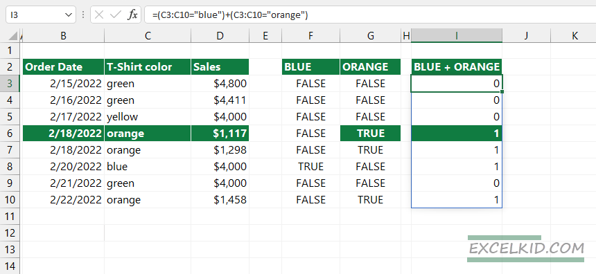
The result is 1 if the cell contains the “blue” OR “orange” value. Now have the lookup array for the second argument of XLOOKUP.
The formula looks like this:
=XLOOKUP(1, {0,0,0,1,1,1,0,1}, sales_data)
Evaluate the formula:
The formula will find the first matching record that meets the boolean or logic criteria. In this case, the first matching record is in row 4.
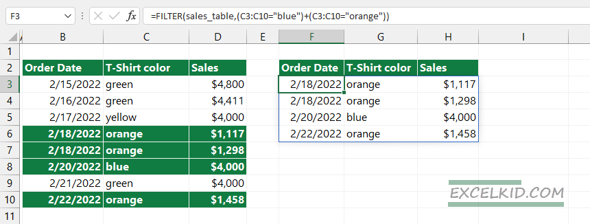
Workaround with the FILTER function
If you want to get all matching records, use the FILTER function.
Formula:
=FILTER(sales_table, (C3:C10=”blue”)+(C3:C10=”orange”))
Result: