Learn how to use XLOOKUP across multiple Worksheets with named ranges instead of the old VLOOKUP function.
Tip: If you frequently work with lookup functions and formulas, we recommend using the most effective solution, XLOOKUP.
LOOKUP Formula in Excel with multiple Sheets
This guide will show you how to summarize information from multiple Worksheets into one Worksheet. The first part of the tutorial will demonstrate the XLOOKUP method with easy error handling. In the second part of the tutorial, we’ll use a VLOOKUP function-based solution. With the help of named ranges, we can simplify the task and make the process easy to understand.
How to use XLOOKUP across multiple Worksheets
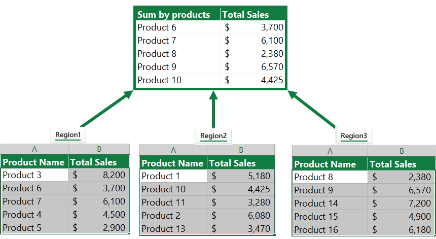
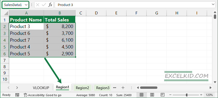
In the picture below, you can see our initial data set, and our goal is to look up values across three Worksheets.
We store the Total Sales in three different Worksheets that contain different products. We’ll use a named range to simplify working with formulas. It is the right decision if you do not want to keep long cell references in mind.
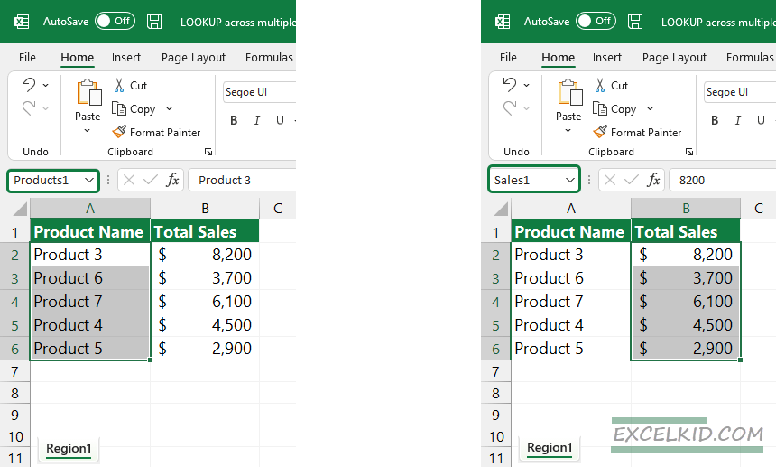
Create a named range
To add a named range, use the steps below:
Select the range you want to describe and enter the name in the name box to create a named range.
This small step saves you time in case of using complex formulas!
Apply names for Worksheet “Region2” and “Region3”.
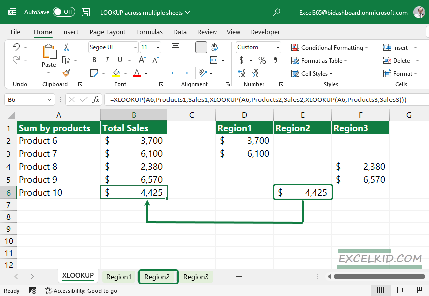
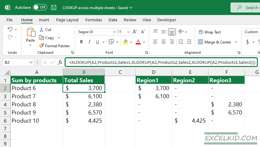
Here is the formula to apply lookup across multiple Worksheets:
=XLOOKUP(A2,Products1,Sales1, XLOOKUP(A2,Products2,Sales2, XLOOKUP(A2,Products3,Sales3)))
Handling the #N/A error
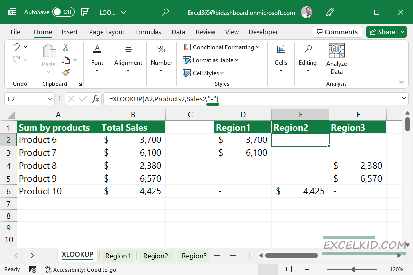
Take a look at the helper table! If you want to validate your formulas, using the 4th argument of XLOOKUP is worth using.
In the example, examine the result of cell E2!
Formula:
=XLOOKUP(A2, Products2, Sales2, “-“)
The formula tries to lookup “Product6” in the Worksheet “Region2”. The formula returns with a text string, “-” if nothing is found.
Next, apply the formula for all cells in the range D2:F6.
It’s easy to check that two values come from the first Worksheet, one from the second, and the last two from the third.
The above-mentioned nested XLOOKUP formula does the rest and returns the proper values.
Workaround with Multiple Worksheets and VLOOKUP
If your Excel version does not support the latest lookup functions, there is a workaround with VLOOKUP. We’ll work with the current example (see above).
Our goal is to use a VLOOKUP-based formula across two Worksheets.
Because VLOOKUP uses different arguments than XLOOKUP, we need to create a new named range.
Formula:
=IFERROR(VLOOKUP(A2,SalesData1,2,FALSE),VLOOKUP(A2,SalesData2,2,FALSE))
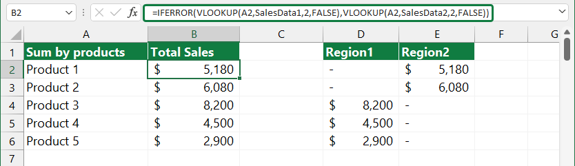
Evaluate the formula from the inside out! We’ll check two cases:
=IFERROR(value if found, value if not found)
=IFERROR(VLOOKUP formula1, VLOOKUP formula 2)
- Case 1: The VLOOKUP function tries to find the lookup value in the second column of the “Salesdata1” range. If an exact match is found, return the value.
- Case 2: If the exact match is not found, the formula jumps to the second Worksheet and lookup the correspondent value for Product1.