Learn how to easily perform a left lookup with the XLOOKUP function instead of using the VLOOKUP or INDEX and MATCH functions.
We already know that XLOOKUP has opened new horizons in Excel. Today’s guide will be on how to replace the VLOOKUP provides limited functionality in case of left lookup.
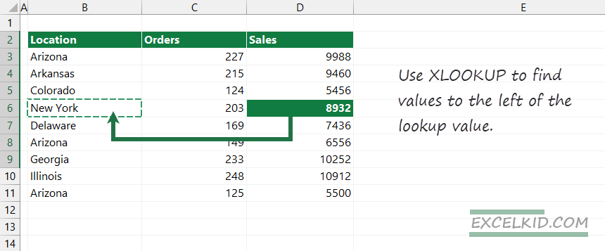
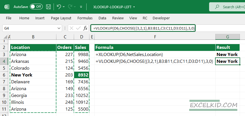
How the left lookup works
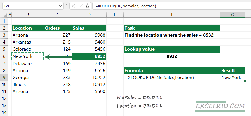
In the example, we want to find the correspondent item in the Location column if the value in the Sales column is 8932.
First, we will create named ranges. This step will dramatically improve the formula’s readability. Select range B3:B11, locate the name box: type ‘Location‘, and press enter. After that, select range D3:D11 and add a name, in this example, ‘NetSales.’
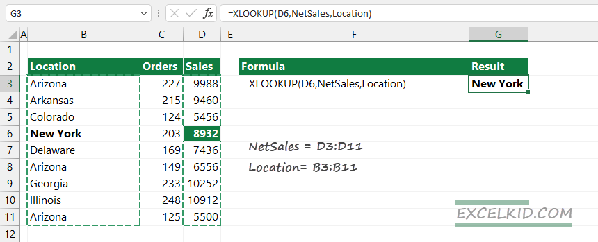
Apply the formula that provides a left lookup:
=XLOOKUP(D6, NetSales, Location)
In the example, we are using the following arguments:
- lookup_value: 8392
- lookup_array: D3:D11 (or a named range, NetSales)
- return_array: B3:B11 (or a named range, Location)
Tip: the formula mentioned above is equivalent to =XLOOKUP(D6, D3:D11, B3:B11)
Workaround with VLOOKUP (reverse lookup)
The most frustrating limitation of VLOOKUP is that the function lookup values to the right only. We need left lookup, so here is a workaround with VLOOKUP.
Using the CHOOSE function, we can rearrange the lookup table:
=CHOOSE({3,2,1}, B2:B11, C2:C211, D2:D11)
=CHOOSE({3,2,1}, Location, Orders, Sales)
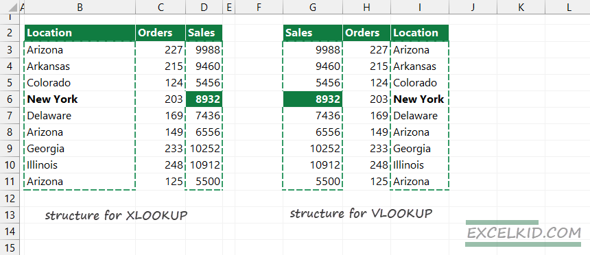
The CHOOSE function rearranges the columns and VLOOKUP using a left lookup.
Inside the formula, CHOOSE swaps columns 1 and 3 and creates an organized table ready for VLOOKUP.
The final formula:
=VLOOKUP(D6,CHOOSE({3,2,1},B3:B11,C3:C11,D3:D11),3,0)
Here is the practice file: