Learn how to create a nested XLOOKUP formula if you need two lookup values to find the matching record in Excel.
We will show you how to use XLOOKUP to replace the INDEX and MATCH combination when you need a two-way lookup. For example, sometimes, we need two inputs to find the matching record in Excel.
Table of contents:
- What is a nested (two-way) lookup in Excel?
- Why is it important to use nested XLOOKUP Formulas?
- Nested XLOOKUP: Using a two-way lookup
- Two-way lookup: Workaround with INDEX and MATCH
What is a two-way lookup in Excel?
A two-way lookup using XLOOKUP refers to a value based on multiple criteria, like a row and a column. The most used scenario is when you have a table and want to find a value at the intersection of a specific row and column. For the sake of simplicity, you have a sales table where the rows represent different products, and the columns represent months. You can use a two-way lookup to find the sales of a selected product in a particular month.
Why is it important to use nested XLOOKUP?
Using nested functions in Excel and specifically nested XLOOKUP is valuable for a few reasons:
- Enable advanced lookups: By nesting XLOOKUP functions, you can achieve more complex lookup scenarios. For example, finding a value in one range and then using that result to look up another value in a different range. This is useful when data is structured so that a single XLOOKUP won’t suffice.
- Improved Formula validation: Working with large data sets, you must validate data in multiple steps to ensure you get the correct information. Using nested lookups helps ensure data accuracy.
- Efficiency: Save your time and use formulas with two-way XLOOKUP. Instead of using multiple helper columns or additional steps, nested XLOOKUP can simplify your formulas and make your worksheet less cluttered.
- Dynamic Data: When working with tables or data that might expand or change over time, nested XLOOKUP can be more dynamic. Furthermore, it is adaptive to such changes, returning correct results even when data is restructured or expanded.
Generic Formula
Here is the generic formula to use a nested XLOOKUP:
=XLOOKUP(row_criteria, row_range, XLOOKUP(column_criteria, column_range, table_range))Explanation: Evaluate the formula from the inside out!
- The inner XLOOKUP finds the correct column based on the column_criteria.
- The outer XLOOKUP finds the correct row based on the row_criteria.
- The selected row and column intersection provides the desired result.
Nested XLOOKUP: Using a two-way lookup
The two-way lookup formula enables you to find and extract the exact match. The point is that we use two variables in the nested XLOOKUP formula.
Before we take a deep dive, create three named ranges:
- Period: C2:F2
- Names: B3: F7
- Sales: C3:F7
Generic formula to apply a two-way lookup using XLOOKUP:
=XLOOKUP(lookup value1, period, XLOOKUP(lookup value2, names, sales)We want to find and get the sales based on two variables in the example. We aim to get the sales if the name is equal to Peter (lookup value1) and the period is equal to Q3 (lookup value2).
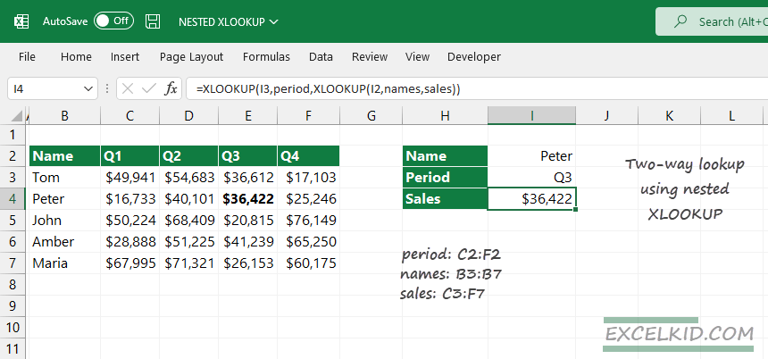
To apply a two-way lookup, use a nested XLOOKUP method. The formula in I4 is:
=XLOOKUP(I3,period,XLOOKUP(I2,names,sales))XLOOKUP performs lookups in horizontal or vertical arrays and returns an entire row or column. We will use this ability in nested XLOOKUP formulas. The formula inside gets the lookup array, and the outer formula will use it as 3rd argument to return the correspondent sales.
Explanation
Let us evaluate the formula from the inside out! First, the inner XLOOKUP formula returns the array where we will find the sales for the given period.
=XLOOKUP(I2, names, sales)The lookup value is in the second row, so the formula will return with the entire row. The result is an array that contains four periods of sales for Peter.
={16733, 40101, 36422, 25246}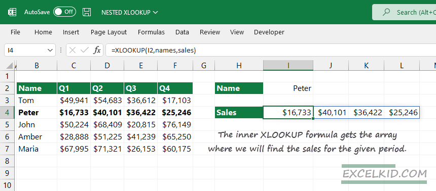
We will use this “return array” as an input for the outer XLOOKUP; the formula will use this array as a third argument:
=XLOOKUP(I2, period, {16733, 40101, 36422, 25246})Finally, the outer XLOOKUP formula finds the lookup value in the third period. The matching value is Q3, so the formula will get the third item in a range.
Alternatively, you can use the nested XLOOKUP without named ranges:
=XLOOKUP(I3, C2:F2, XLOOKUP(I2, B3: F7, C3:F7)Two-way lookup: Workaround with INDEX and MATCH
If your Excel has no XLOOKUP support, you can perform a two-way lookup using the well-known INDEX and MATCH combination.
Formula:
=INDEX(C3:F7,MATCH(I2,names,0),MATCH(I3,C2:F2,0))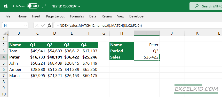
Explanation:
=MATCH(I2,names,0) //2nd row
=MATCH(I3,period,0) //3rd column
=INDEX(C3:F7,2,3)
Nested XLOOKUP: Create the lookup value
We used the inner formula to get the lookup array in the demonstrated formula above. We aim to find the total cost in the second table where the Product is “Banana” in the first table. As usual, we will use named ranges in case of advanced formulas.
We need to find the link (Product ID) in the first table and then use it as a lookup value in the outer lookup formula.
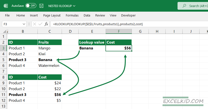
First, use a left lookup in the first table to get the correspondent ID.
=XLOOKUP($E$3,fruits,products1) //Product3We will use the result –Product 3– as the lookup value for the main formula. Apply “Product 3” as a first argument to find the matching record in the second table:
=XLOOKUP(F3,products2,cost)Replace F3 with the original formula; here is the nested XLOOKUP formula that supports two-way lookups:
=XLOOKUP(XLOOKUP($E$3,fruits,products1),products2,cost)Related Formulas: