Find the 2nd match using XLOOKUP

This guide will explain how to find the 2nd match or the nth occurrence in an array using the XLOOKUP function.

There is a common problem with all lookup functions in Excel: how to skip the exact match and get the 2nd, 3rd, or nth match. We will use the XLOOKUP function in the example to find the second or nth occurrence. In the second part of the article, we’ll demonstrate the method to get the nth occurrence in case of multiple lookup values.

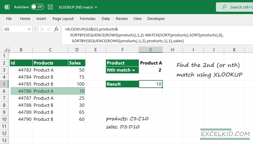
Find the 2nd match using XLOOKUP

Our table contains three columns: ID, Products, and Sales.

In the example, we use named ranges:

• Products: C3:C10
• Sales: D3:D10

We want to lookup Product A in column C and return the corresponding Sales from column D.
Let’s find the 2nd occurrence for Product A and get the matching sales.

Formula to find the 2nd match using XLOOKUP

By default, XLOOKUP returns the first matching record. What if we want to find the second match? The following formula uses some tricks:

=XLOOKUP(lookup_value&2, lookup_array&nth_lookup_array, return_array)

Okay, at first glance, a bit of explanation is necessary. So, we’ll explain the concept before we examine the formula. We use only the first three (required) arguments in the example.

Construct the lookup value and lookup array:

To create the lookup value, we need to use an ampersand (&) between the Product name and the nth parameter.

Lookup value if we are looking for the second match for Product A:

= Product A&2 = G2&G3 = ProductA2

Create the second argument of the XLOOKUP function: the lookup array. So, we will build a temporary array that gets the nth occurrence number of the lookup array items. To do that, use a formula based on the SORTBY, SEQUENCE, and ROW functions.

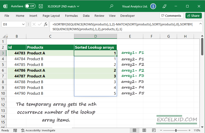
Formula to get the temporary array that contains a sorted list for all lookup values:

=SORTBY(SEQUENCE(ROWS(products),1,2)-MATCH(SORT(products),SORT(products),0),
   SORTBY(SEQUENCE(ROWS(products),1,2),products,1),1),sales)

In column E, you can identify the position of the lookup value in a lookup array even if you have different types of products. Finally, XLOOKUP will use the result of the SORTBY formula as a lookup array. The last part of the formula is the return array. We want to know the sales, so use the sales range (C3:C10) as a return array.

=XLOOKUP(G2&G3, products&
  SORTBY(SEQUENCE(ROWS(products),1,2)-MATCH(SORT(products),SORT(products),0),
  SORTBY(SEQUENCE(ROWS(products),1,2),products,1),1),sales)

Download the practice file!

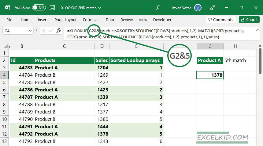
Formula to find the nth match in a range

Now, we can easily find the 2nd match using the formula mentioned above. What if we want to find the 3rd, 4th, or nth occurrence using XLOOKUP?

Generic formula to find the nth match in a range:

=XLOOKUP(lookup_value&nth, lookup_array&nth_lookup_array, return_array)

The good news is that the formula is flexible; replace the lookup value with the preferred value, and you will get the nth match.

Get the 2nd, 3rd, or nth match for multiple lookup values

This chapter demonstrates how to create the lookup value if you want to use multiple lookup values in a single formula.

It’s good to know that we can leave the lookup_array and return_array parts untouched. The point is that using a range as a lookup value then concatenates the nth position.

In the example, we want to find the 2nd match for Product A and Product B simultaneously using one formula.

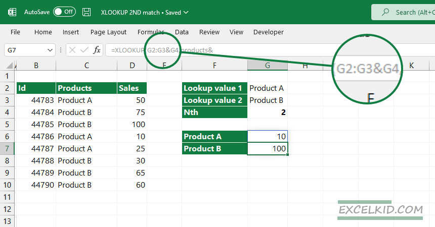
The lookup_value is a spilled array:

=G2:G3&G4

We recommend you check the practice file and take a closer look at the formula. Stay tuned.

Additional resources:

• How to get all matching results using lookups