Excel Transpose Function

The Excel TRANSPOSE function swaps a vertical range to a horizontal range and switches rows to columns but keeps the data structure.

Table of contents:

• Convert rows to columns in Excel using Transpose
• Excel Transpose Shortcut
• How to use Excel Transpose Function
  • Steps to convert rows to columns using Array Formula
  • Transpose data in Excel using Office365 (Microsoft 365)
• Convert rows to Columns (VBA solution)
• Transpose Data using PowerQuery
• Excel Online (Web) Script

Convert rows to columns using Transpose

In this tutorial, you will use the Paste Special command menu to transpose data in Excel.

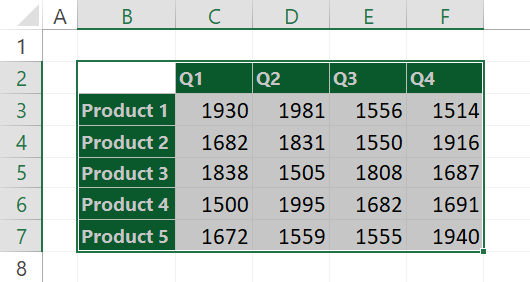
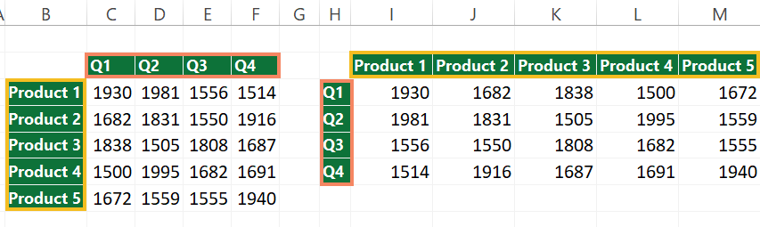
Our table contains sales data: products, period, and sales.

1. Select the range (rows and columns) that you want to transpose. Then, copy the data to the Clipboard using the Ctrl + C keyboard shortcut.

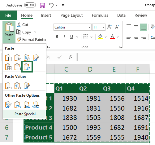
2. Select the Home Tab and click the Paste option. A drop-down list appears that contains some paste options.

3. Select the target cell where you want to place the transposed data. The selected cell will be the top-left corner of the transposed data.

4. Click on the Transpose icon to paste the data.

Transpose Excel Shortcut

The demonstrated method will help you to perform the task using shortcuts only!

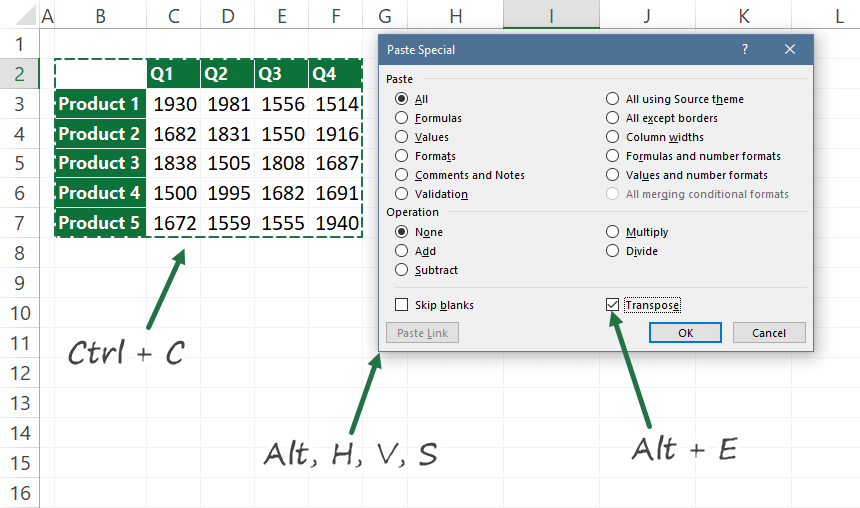
1. Select the source range, then use the Ctrl + C shortcut
2. Select the target range, then apply the Alt, H, V, S shortcut to open the Paste Special dialog box
3. Check the Transpose option manually, or use the Alt + E shortcut to select the Transpose checkbox.
4. Press OK to paste the data

How to use Excel Transpose Function

The Excel TRANSPOSE function converts a vertical range of cells to a horizontal range of cells. It’s a reverse function, and you can convert a horizontal range of cells to a vertical range of cells.

In other words, the TRANSPOSE function replaces the orientation of a given range or array:

• If you have a vertical range, TRANSPOSE converts it to a horizontal range
• In the case of horizontal range, TRANSPOSE converts it to a vertical range

Good to know: The transposed range is dynamic. What does this mean in practice? If you change one or more values in the source range, the Excel Transpose function will update the target range data.

Steps to convert rows to columns using Array Formula

Use this method if you are working with Excel 2013, Excel 2016, or Excel 2019.

In the first example, take a closer look at the range B2:F7! The range, in this case, is a 6×5 matrix. You want to change the orientation and convert the selected cells into a horizontal array. So, you must choose a target range containing five rows and six columns.

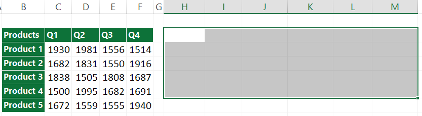
1. Select the target range; in this case H2:M6

2. Go to Formula Bar and enter the formula:

Use the =TRANSPOSE(B2:F7) formula, but don’t hit Enter. Instead, use the Ctrl + Shift + Enter keys to create an array formula.

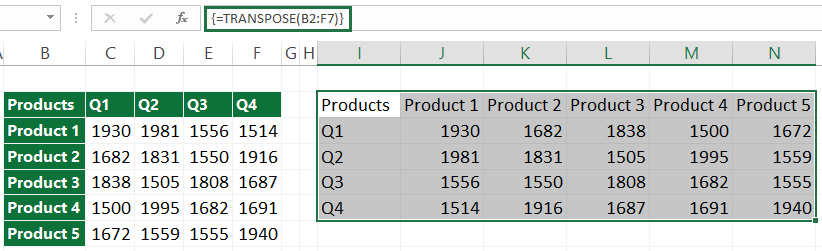
You will get the result quickly after pressing the Ctrl + Shift + Enter. When you see curly brackets around the formula, the transformation was successful. These curly brackets are how Excel recognizes an array formula.

Transpose data in Excel using Office365 (Microsoft 365)

We strongly recommend you use the latest Excel; now, you will learn why. In addition, the simplified Transpose Excel function provides time-saving tricks.

Differences between old and spilled array formulas in Excel: Legacy array formulas (you can find them in older Excel versions) always return a fixed-size result. However, when you press Enter to confirm the Transpose formula in the latest version of Microsoft Excel, Excel will dynamically size the output range and place the results into each cell within that range.

Let us see how the spill feature works:

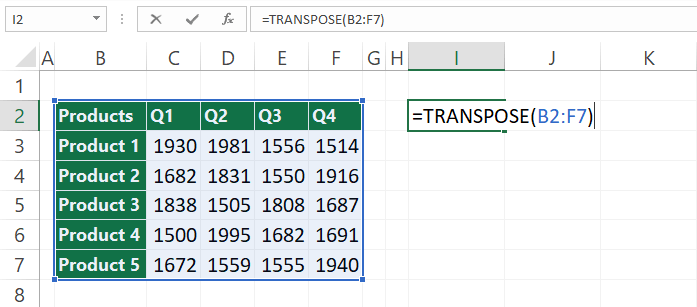
Select cell I2, then enter the range that you want to transpose.

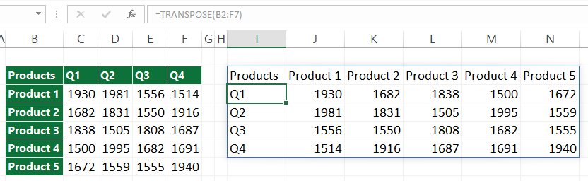
Press Enter!

If you are working with the latest Excel, using the curly bracket and the Ctrl + Shift + Enter keystroke is unnecessary.

Once you enter a spilled array formula, Excel will place a highlighted border around the transposed range when selecting any cell within the spill area. The blue border will disappear when you select any cell outside of the transposed range.

What a great feature: paste a range into a single cell.

Good to know: Excel still supports the old Ctrl + Shift + Enter method for backward compatibility reasons.

Convert rows to Columns using Transpose (VBA solution)

You can write macros if you are familiar with Visual Basic for Applications. Then, run the macro from the Developer Tab or place it in the Quick Access Toolbar.

Use the Alt + F11 shortcut to open the VBA editor window. Then, copy the code below into a new module.

Sub QuickTranspose()
    Dim vFormulas As Variant
    Dim oSel As Range
    Set oSel = Selection
    vFormulas = oSel.Formula
    vFormulas = Application.WorksheetFunction.Transpose(vFormulas)
    oSel.Offset(oSel.Rows.Count + 2).Resize(oSel.Columns.Count, oSel.Rows.Count).Formula = vFormulas
End Sub

If you are using the Transpose function frequently, add the macro to the QAT.

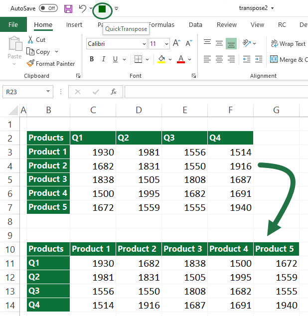
In the example, you can use the Alt, 4 shortcut to transform your data.

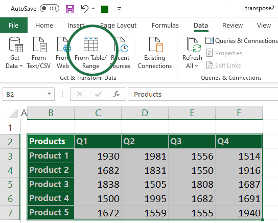
Transpose Data using PowerQuery

When you store data in an Excel Table and you need to use the transpose function frequently, follow this guide.

1. First, select the range that you want to transpose. Locate the Data tab on the ribbon and use the From Table/Range function.

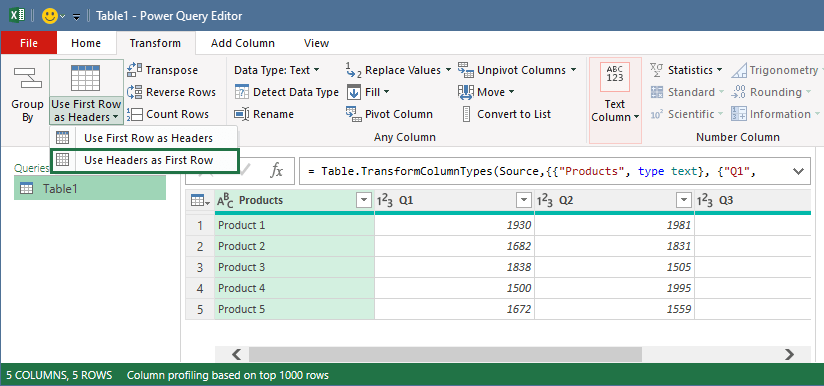
2. The Power Query editor window will appear.

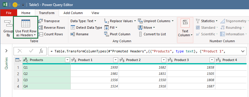
3. Select the Transform tab, and click on ‘Use Headers as First Row’ from the ‘Use First Row as Headers’ drop-down list.

Select the Transform tab in the Power Query Editor and use the Transpose command to convert rows to columns.

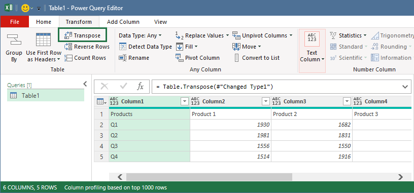
Once Excel transposes the data, you need to switch the column header back. To do that, select the Use First Row as Headers to promote the first row of this table into column headers.

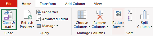
Now, you want to get back to Excel and check your data. But first, go to the Home tab and click on the Close and Load button.

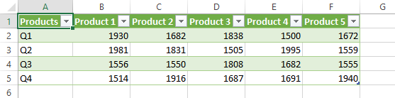
Excel will place the transposed data into a new Worksheet.

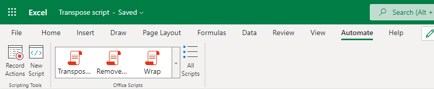
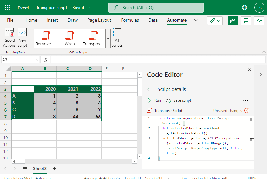
Excel Online (Web) Transpose Script

If you are working with the web version of Microsoft Excel, you can use the typescript language to create simple and complex scripts.

Locate the Automate tab on the ribbon and click on New Script to reach the Code Editor on the right pane.

Insert the following script. The script will transpose the selected range and then paste the data to the range that is started with cell F3.

function main(workbook: ExcelScript.Workbook) {
  let selectedSheet = workbook.getActiveWorksheet();
  selectedSheet.getRange("F3").copyFrom(selectedSheet.getUsedRange(), ExcelScript.RangeCopyType.all, false, true);
}

Finally, add a new name, then save the script.

Run the script and convert rows to columns quickly! The script will place the converted range, starting with cell F3. You can easily change this parameter to place the get result in another sheet or range.

Wrapping things up

• Use dynamic arrays if you are working with the latest Excel, Microsoft 365
• Remove filters before applying Transpose
• Use the Quick Access Toolbar to speed up your work
• If it is possible, use shortcuts
• If you have large data tables, use Power Query

Here is a video tutorial:

Additional resources

• Wrap Text in Excel
• Excel Functions