Using the drop-down list, we can choose elements from a predefined list. It is beneficial when, for example, we would like to show the efficiency of different departments within one company. Moreover, it is worth using because when choosing its elements, the dashboard automatically refreshes and, likewise, the connecting charts.
Forget all user-generated errors! Drop-down lists help us to avoid incorrect data entry! In the first example, you’ll learn how to create a drop-down list. After that, we will introduce the conditional drop-down list. Finally, we’ll show you how to use our free add-in to create a drop-down list using dynamic named ranges.
We cannot press it enough times to save considerable space, which is a great value when creating an Excel dashboard or a dynamic chart.
Steps to create a quick drop-down list
It’s a simple process to create this data validation feature. Because data validation is a built-in feature in Excel, we’ll create a list (source data) and an input cell for data entry. The tutorial shows how to implement a drop-down list in a Worksheet.
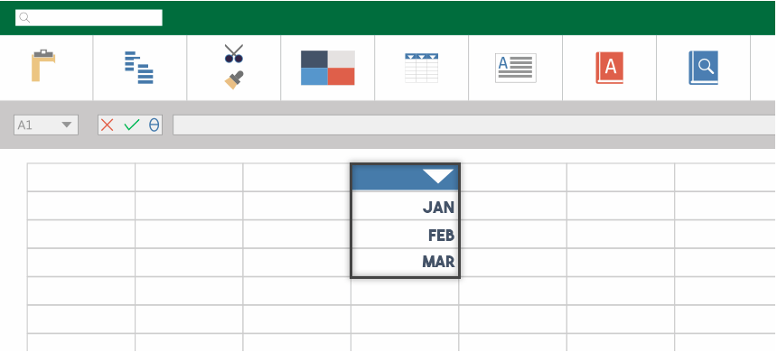
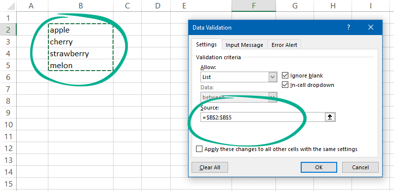
Click the drop-down list to display items from “B2:B5”. We cannot enter a new record if we try to enter something that isn’t on the list. That’s the point!
To create a drop-down list for a Worksheet, follow these steps:
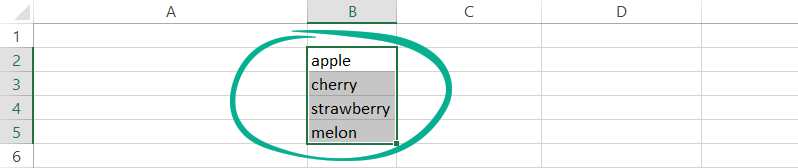
1. Set up the list first. Create the list in cells B2:B5. You can choose a row as a range, for example, B2:E2. In this case, you should use the transpose function.
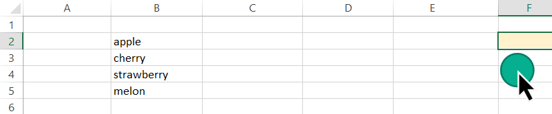
2. Select the position of the drop-down list in the example, cell F2.
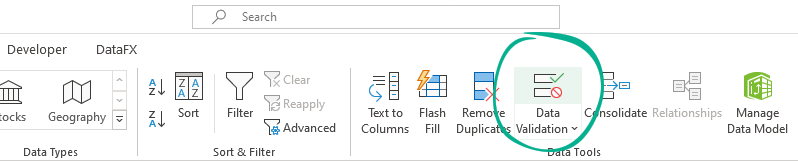
3. To apply data validation to cells, jump to the Data Tab and select Data validation.
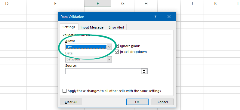
4. Add data validation criteria! Select ‘List’ from the drop-down menu.
5. Click ‘Source’ and select the range B2:B5 to add a data source. Next, select the in-cell drop-down checkbox. Finally, make sure that the in-cell Drop-down option is checked.
6. Click OK, and the list is ready to use.
Build a conditional (dependent) drop-down list
Sometimes, we want to use the conditional drop-down list.
Explanation: We have two lists, and the items appear in the second drop-down list, depending on the selection we built in the first menu. This solution can be useful if you want to use classification in Excel.
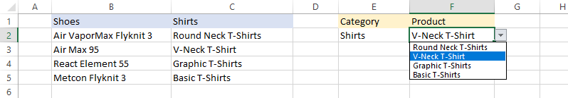
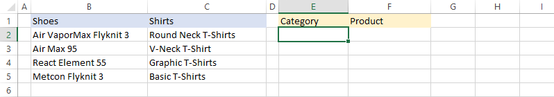
For example, the first list contains 4 kinds of shoes; the second includes 4 types of t-shirts. We want to divide all the elements into two sections: Shoes and Shirts. The first list is the category selector. You can choose only those elements from the second list, dependent on the first selection.
The options in the Products depend on the selection applied in the category. For example, if you choose ‘Shoes’ in List 1, you’ll see the shoe types. If you select ‘Shirts’ in List1, Excel will display the shirt types in the Product list.
Steps to create a dependent drop-down list in Excel
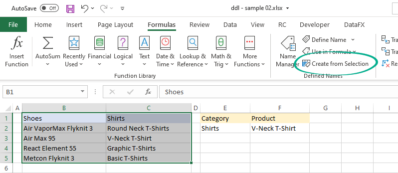
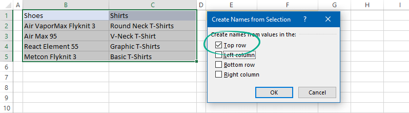
Select the list headers and create names from the selection. This function generates names from the selected cells automatically.
The ‘Create Named from Selection’ dialog box appears. Check the Top row option only. Click OK.
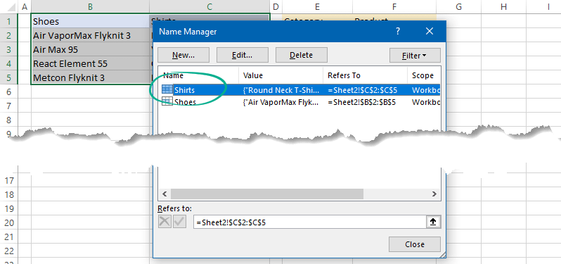
Now we have two named ranges (‘Shirts’ and ‘Shoes’). Shirts named range refers to all the shirt types in the list. Shoes named range refers to all the shoe types in the list.
Select cell E3 to place the first menu.
To display the data validation dialog box, go to the Data Tab and choose Data Validation.
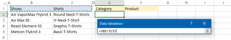
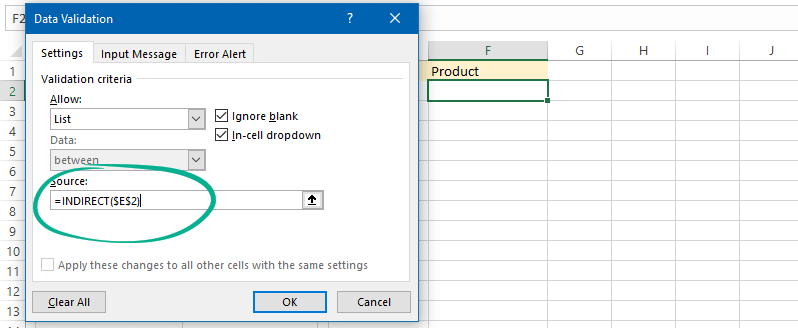
Select the list in the data validation on the Settings tab. The source range is B1:C1.
Click OK. Select cell F2 and apply data validation to create a second drop-down list.
Use the formula below.
=INDIRECT($E$2)
Finally, click OK.
Error handling using INDIRECT and SUBSTITUTE formulas
Explanation of INDIRECT formula:
The INDIRECT function gets the reference specified by a text string. For example, if we select Shoes from the first list, the formula ‘=INDIRECT($E$2)’ returns the second list containing the shoe types.
We want to avoid some frustrating errors regarding multi-word category names. For example, if we create a two-word category, ‘Running Shoes’ instead of ‘Shoes.’, we must apply a different formula. In this case, we should use a combination of the INDIRECT formula and SUBSTITUTE formula.
Keep in mind that using spaces in named ranges is not allowed.
The best solution to convert spaces into underscores:
=INDIRECT(SUBSTITUTE($E$2,” “,”_”))
This formula will replace the spaces and help to prevent unwanted issues.
A faster way to create a drop-down list
If you are in a hurry, we can help you! First, install our spreadsheet tools and create a drop-down list using a single userform. (The add-in will be available in a few days!)
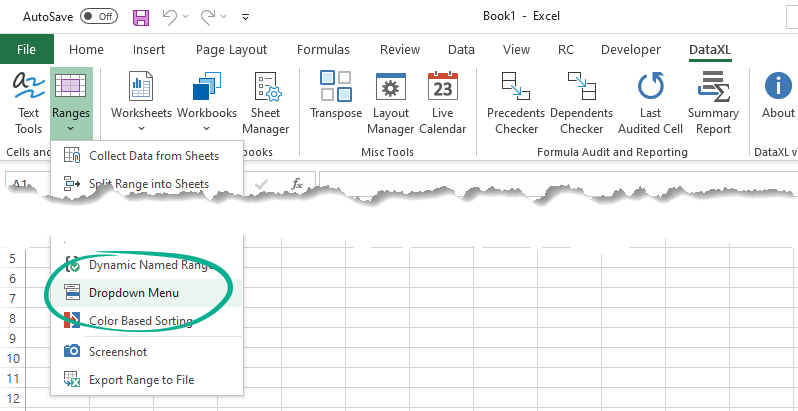
First, please check and enable the developer tab if it does not appear. Then, go to the DataXL tab on the ribbon and choose the drop-down list icon from the Cells group.
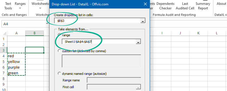
A small popup window will appear—for example, select cell B2 to place the list. Now, choose the data source. You have two options: use a predefined range or create a custom list.
The following example will show you how to create a drop-down list using comma-delimited text.
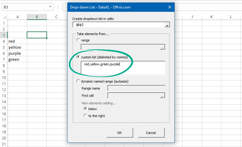
The result is the same.
Conclusion
Drop-down lists are helpful to select an item from a fixed list. It’s an effective way to create forms using a graphical way, forcing users to choose a value from a list.