
Use Excel Tables to simplify your work! Learn how to create dynamic ranges, easy-to-read formulas using a table. In this tutorial, we’ll explain how to add new data to a range or how to manage Tables. Keep your formulas ready for auditing!
This guide provides useful tricks and examples.
- Fundamentals of Excel Tables
- Working with Tables
- Table Formatting
- Tables and Data sources
- Convert Excel Tables to a normal range back
Fundamentals of Excel Tables
In this section, we’ll start with the basics.
Creating an Excel Table is Easy
How to create an Excel table?
- Select the range which contains data.
- Use the insert Table keyboard shortcut, Control + T
- If your table has headers, select the ‘My Table has headers’ checkbox.
- Click OK, and Excel will create a new table.
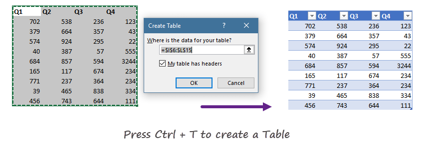
If you are in a hurry, Excel Tables is yours! On the right side of the picture, you’ll see banded rows.
Rename a Table
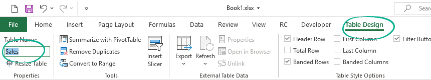
When you create a new Excel Table, Excel will assign a custom name, like Table1. You have to rename it and add a short, user-friendly name like ‘Sales.’
Important: Each table must have a unique name that contains letters, numbers, or the underscore character (for example, using spaces or special characters between words is not allowed.
To change the default name, select your table and locate the Table Design Tab. Jump to the Table Name > Properties section. Add a new name and press Enter.
The Parts of a Table
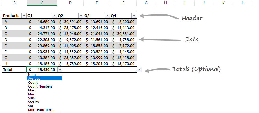
All Excel Tables have two required and one optional part.
The Column Header Row is the first row of the table. It contains identifiers, for example, ‘Product,’ ‘Order Date,’ and so on.
The body is the main data set.
Optional: you can switch an additional (Totals) row using the ‘Ctrl + Shift + T‘ shortcut.
Navigating between Tables
If you want to find your table quickly, locate the Name Box and use the drop-down menu in the top-left area of your workbook. Choose the table name, and what you want to activate. The range will be highlighted.
What if your table is located in a different tab? Excel will jump to the selected table.
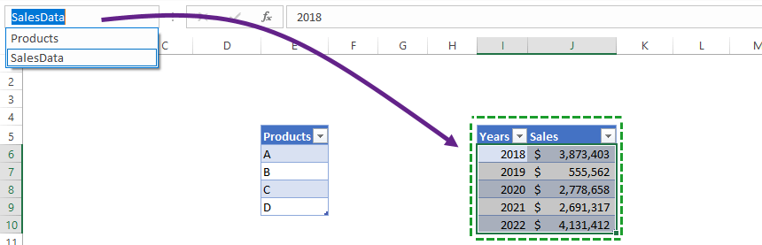
Table related Shortcuts in Excel
If you have tabular data, you can easily convert it to an Excel Table.
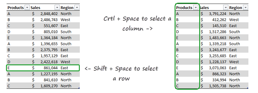
If you select a simple cell in the table, you can select the actual row using the ‘Shift + Space’ command. To select rows, use the ‘Control + Space’ keyboard shortcut.
Working with Tables
Moving Excel Tables
The easiest way to move a table to a new location is using a drag and drop method with a mouse.
In the example, we’ve just selected the original table then moved it to the K4:N13 range.
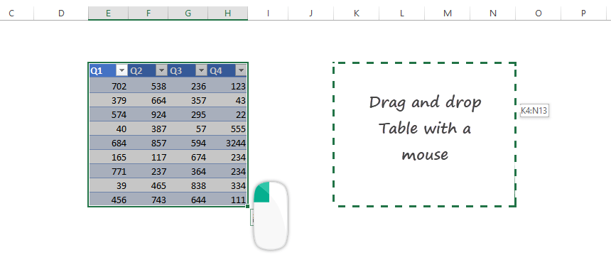
Tip: This is the fastest way to move tables to a new location. The method works only on the same sheet!
Swapping rows or columns in the table
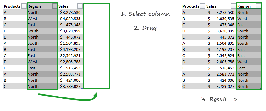
It can frequently happen that you want to change the table structure or swap rows or columns. As first, select the table row or a table column. Make sure that the header row is selected. Drag the selected range and drop to a new area.
Excel will swap the given rows or columns. The method is safe because Excel will not overwrite the existing data.
Keep Table headers always on the top
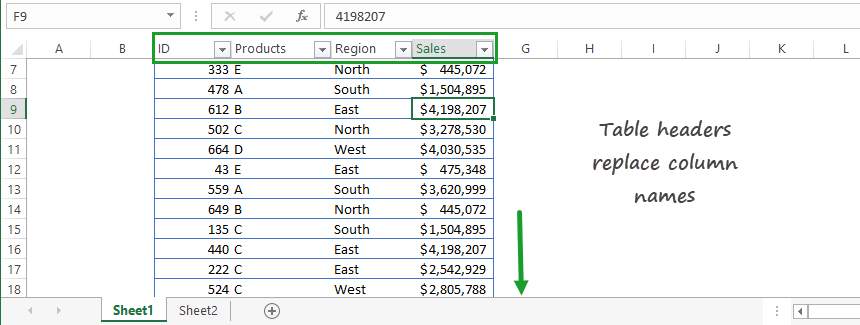
Excel Tables work simply. Are you working with large data sets? No problem! You can scroll down without any trouble. The table header will stay on the top. It’s not necessary to use the good old Freeze Top Rows function.
You can find it under the Freeze Panes group.
Expand your Table easily
In some cases, you need to insert rows or columns into an Excel Table. We’ll show you how to do that. The Excel Table is a dynamic range; it will resize even if you add or delete rows or columns.
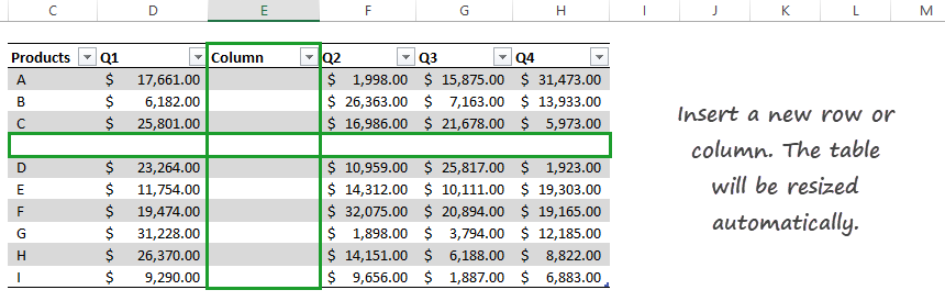
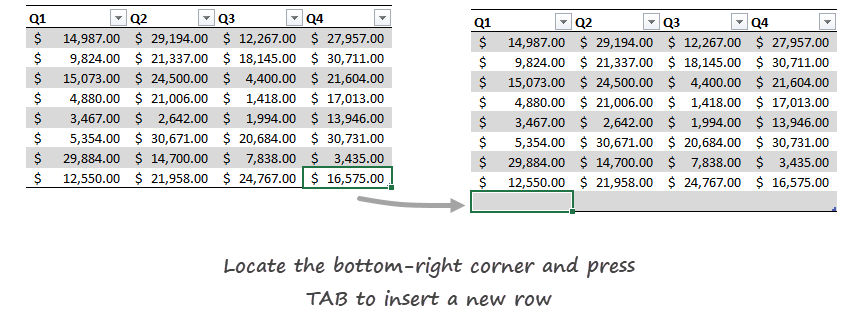
To add a new row, select the bottom-right cell in the range, in this example, cell F11. Press the Tab button; a new row appears, and the table structure remains.
It’s not necessary to select the range and add a new name for a range again.
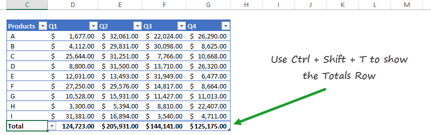
Show Totals (Sum, Count, Min, Max) without using formulas
With the help of tables, it’s easy to show dynamic Totals. Use your preferred formulas, like SUM, COUNT, AVERAGE, MIN, and MAX. Good to know that you don’t have to enter these formulas manually. Great!
You have a filtered Excel table on the left side and a regular table on the right side in the picture below. Use the ‘Control + Shift + T‘ shortcut to display the additional row under the table.
Resize an Excel Table
In the example below, you’ll learn how to change the table size using the ‘Resize Table’ command. This function is yours if you need to prepare a table for – for example – 500 rows.
To resize a table, select the new data range for your table. Click the OK button.
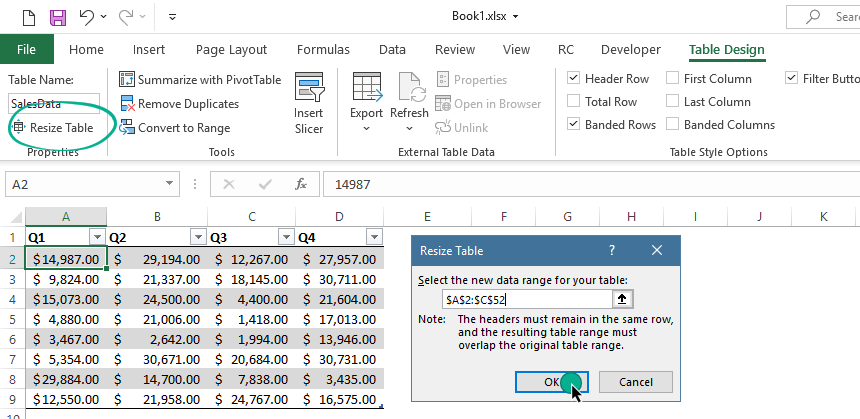
Note: The table headers must remain in the same row, and the resulting table range must overlap the original table range.
Or you can use the classic resize on the fly technic too. Select the small green triangle keeping the left mouse button pressed.
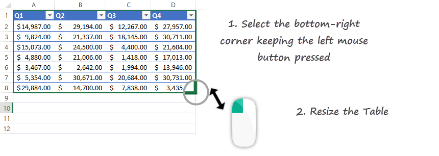
Table Formatting
Change table formatting quickly
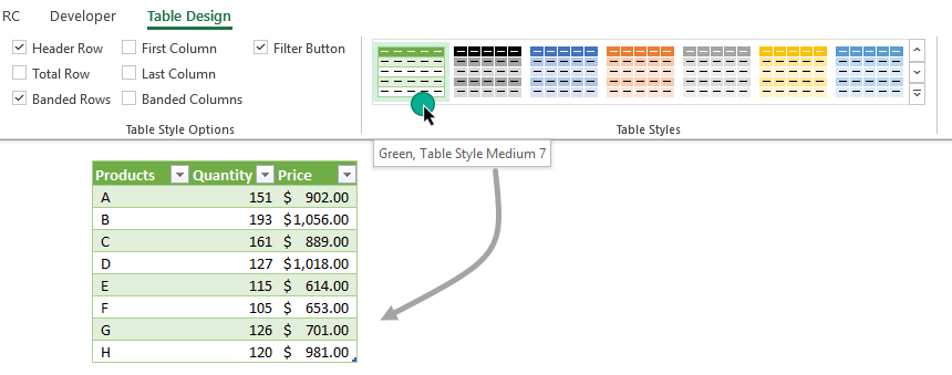
When you create a new table, it has a default formatting style. To override the displayed theme select a cell in the range. Choose the Table design tab on the ribbon and locate the Table Styles Group.
Click your preferred style, and the new theme will appear with a single click.
If you want to use the classic style without formatting, select the table and choose the default style by clicking on the top-left corner of the table style previews. The name of the first style is ‘None.’
Choose your Table style
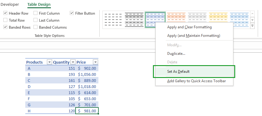
You can choose a default table style. What is the default style? Start Excel and create your first table. Excel assigns a built-in style to the table.
Select the style that you want to apply to all new tables in the future. Right-click on the Table preview and click on the ‘Set as default’ option.
Learn more on how to remove table formatting in Excel.
Tables and Data Sources
Quick Analysis works with Excel Tables
Everyone knows that the Quick Analysis Tool is a great function in Excel. Create your table first. After that, click Control + Q to create a floating row like in the picture below:
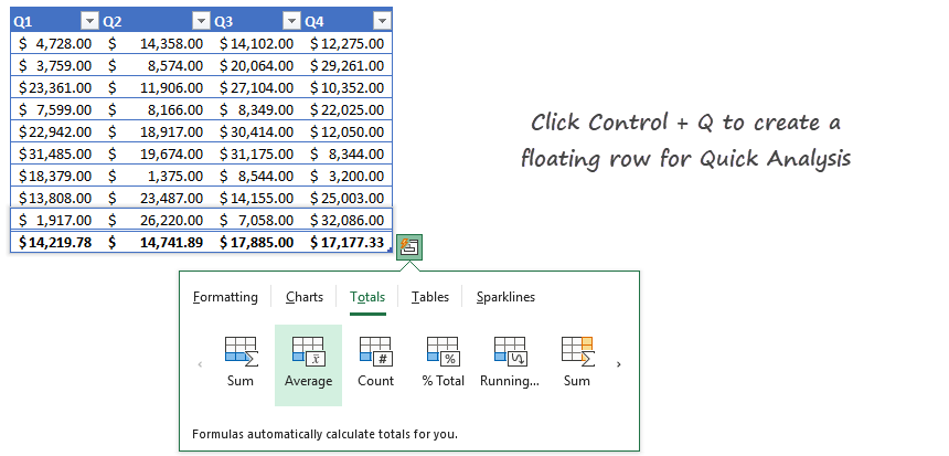
Apply various methods to analyze your data. Use conditional formatting, create chars, or calculate Totals, among others. If you need more power, use conditional formatting.
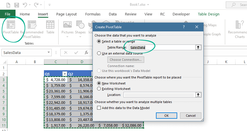
Use a Table as a pivot table source
Is it possible to use an Excel table as a pivot table source? Absolutely.
As we mentioned before, the Pivot table will track the changes in the table. If you add new data to the range, the pivot table will refresh automatically.
Go to the Insert tab. Insert a new pivot table.
A new window appears. Select the data that you want to analyze.
Finally, click OK.
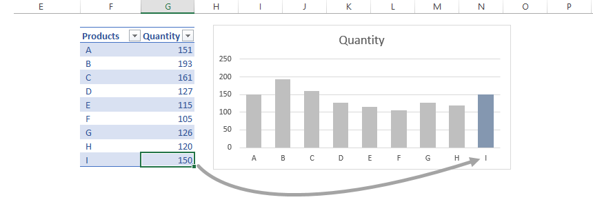
Build dynamic charts using Excel Tables
In our latest article, we’ve just talked about dynamic charts.
If you update your data frequently (adding rows or columns), tables are great for these purposes. Put your fresh data into the table, and the chart will refresh using the entered values.
Insert a new slicer into a table
Good to know that all Excel Tables are slicer-ready? What does that mean in practice? Slicers are special filters. With its help, you can filter data quickly in various ways.
To add a new slicer:
- Select the table
- Locate the Table Design tab on the ribbon
- Locate the Tools group and Click the Insert Slicer button.
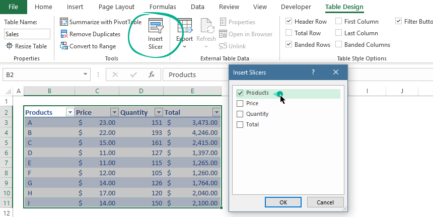
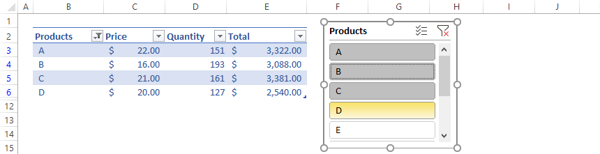
In the example below, now we have a slicer for Products:
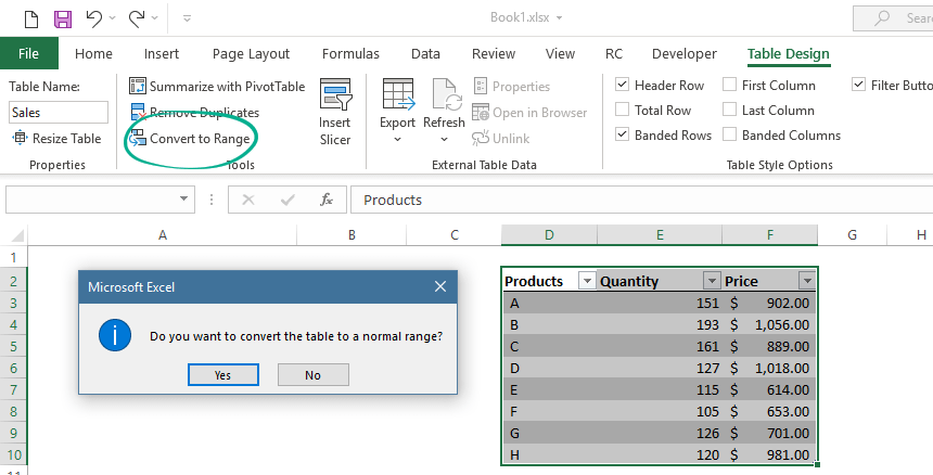
Convert Excel Tables to a normal range back
Tables are useful, but sometimes you need to work with normal ranges. To convert an Excel Table into a range back, do the following steps.
- Select the Table
- Remove the formatting style (choose the ‘None’ table style)
- Click on the Table Tools Tab
- Apply the ‘Convert to Range’ commands.
Note: Step 2 is necessary; otherwise, the formatting styles remain.
Conclusion
Excel Tables are versatile tools. With its help, you can speed up your daily tasks.
You May Also Like the Following Excel Tutorials:
- Creating an Excel Dashboard – The Ultimate Guide
- Structured references