Excel structured reference is a syntax that applies table names in easy-to-read formulas instead of regular cell references.
Use this tutorial to discover the basics of Excel structured references. We will share the details if you are working with tables and Excel Formulas.
Table of contents:
- What are structured references in Excel
- How to create an Excel structured reference
- Structured reference syntax
- Formula examples
- Calculated columns
- Excel auto-update cells after changing Formulas
- Build easy to read Formulas using structured references
- Benefits of using dynamic ranges
- Enter structured references using autocomplete function
- Build structured references using on-the-fly selection with the mouse
- Absolute and relative references
What are structured references in Excel?
A structured reference makes it easier to use formulas with Excel tables by replacing cell references such as F2:F6 with predefined names – like [Q4 Sales] – for the items in a table.
It is good to know that the table reference is dynamic. The reference changes when you add or remove data from an Excel table or drag and drop the table.
Here is an example that shows you the differences between range reference and structured reference:
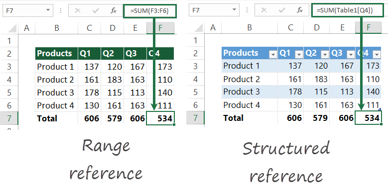
To sum a specified column, the formula is:
=SUM(table name[column id])To count all items in the given column, use the following formula:
=COUNTA(table name[column id])where column id is the name of the column. If you are unfamiliar with dynamic ranges, read our definitive guide on creating an Excel Table.
How to create an Excel structured reference
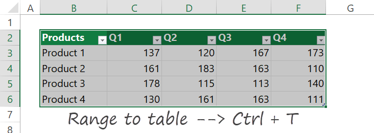
First, you should know how to create a table from a range.
Select the range and use the Ctrl + T shortcut.
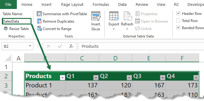
If you want to make your work faster, add a name to the table. First, select the Table Design Tab. Next, locate the Properties Group and type a name, in this case, ‘SalesData.’
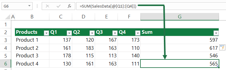
Because you want to sum the yearly sales data for each product, add a new column name in cell G2, and Excel will append the range automatically.
Here are the steps to create a structured reference:
1. Start writing the formula using an equal sign and the SUM function.
2. Select the range from cell C3 to F3 using the mouse.
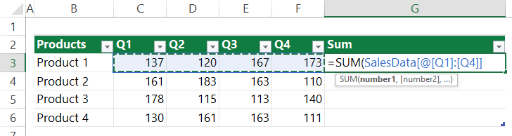
3. After pressing Enter, Excel will apply the autofill feature and copy the formula until cell G6.
=SUM(SalesData[@[Q1]:[Q4]]In this case, Excel will calculate each row individually.
Structured reference syntax
In this section, you will learn how the structured reference syntax works.
What’s the point? A structured reference is an expression that begins with a table name. Furthermore, the end of the formula contains a column specifier.
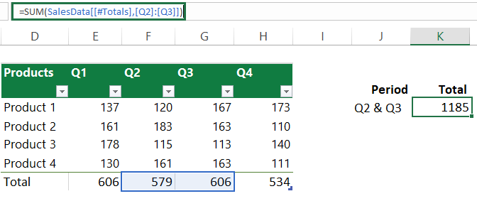
In the example, the formula summarizes the totals of the Q2 and Q3 columns in the table named SalesData.
The main components of the structured reference:
- Table name: SalesData
- Item specifier: [#Totals]
- Column specifiers: [Q2]:[Q3]
Select the cell that contains the formula, and then Excel will highlight the referenced table cells:
The table name indicates only the data, without header row or total rows. If you want to add a name, click on the Table Design tab.
The column specifier points to the corresponding column without the header and total rows. It uses the column name between brackets, like [Q2]. If you are using ranges, the syntax is [Q2]:[Q3]
To point to specific parts of a table, use an item specifier. Here is a list of variables:
- [#All]: Entire table
- [#Data]: Data range
- [#Headers]
- [#Totals]: Total row
- [@Column_Name]: Current row
Formula Examples
In this section, you will find various examples! But first, look deeply into the dynamic ranges and structured references.
Calculated Columns
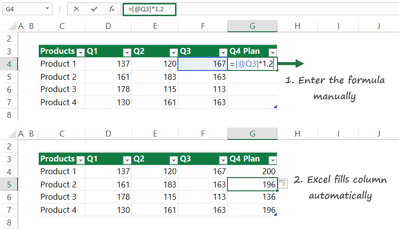
Managing formulas has never been easier! The calculated columns function makes your work more accurate. Let’s see an example:
Try to enter a simple formula in a column. Now press Enter, and the Excel will populate the table automatically. It’s excellent for auditing purposes; you don’t have to copy the formula manually.
The result looks great, and it is error-free.
Excel auto-updates cells after changing Formulas
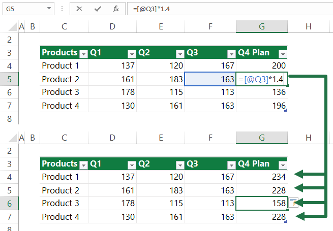
Let us assume that you need to change the formula in the calculated column.
What will happen?
Update the formula in an arbitrary cell in the calculated column. Changes in any rows are propagated to all banded rows. Thus, in the example below, the formula will change the planned sales to 40% in one step.
Build easy to read Formulas using structured references
Are you in trouble with the spreadsheet audit? Sometimes, an audit can be painful when you are working with complex formulas. Structured reference is a great Table feature; it uses easy formula syntax to point to a part of a table.
You will learn how to use a formula outside the table in the example. However, for the sake of simplicity, you want to calculate the total sales. Therefore, if you are working with normal ranges, the formula will be:
=SUM(D4:G7)If you have a table, work with structured references! The formula looks like this:
=SUM(SalesData)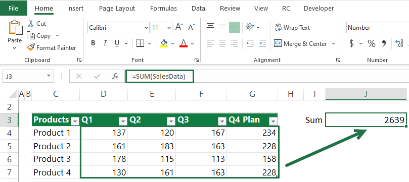
1. Select the cell where you want to place the formula. After entering the SUM formula, press the first character of your table name. Excel will show a drop-down list. Select ‘SalesData’. Double-click on it!
Benefits of using dynamic ranges
As stated above, the most significant advantage of using tables is that we can automatically expand the table with new records. So, the Excel table is a dynamic range!
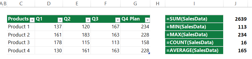
OK, it’s time to learn how to use our formulas with a dynamic range. In the example, locate the table named ‘SalesData.‘
As usual, you can use your formulas to add the table name as a parameter. If you add new records, the formula will refresh the range and modify the result.
Enter structured references using the autocomplete function
If you want to speed up the data entry, use the Excel auto-complete function. Try to start typing the table names. After entering the first character, a floating window appears. Select the correspondent table name from a drop-down list.
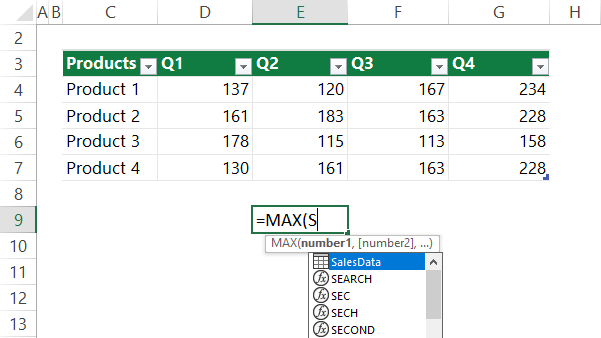
To move the list up or down, use the arrow keys. Next, select and confirm the table name using the Tab button. The trick works fine with the Table columns, too.
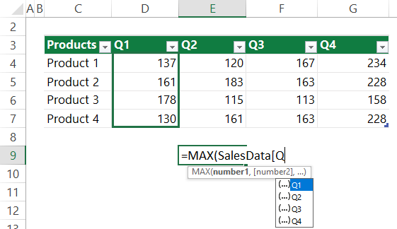
In the example above, we’ve just entered the Table name. Next, let’s see how to calculate the maximum sales amount in Q1 using structured reference.
To refer to a column, open a bracket by typing a ‘[‘sign. The autocomplete trick, as mentioned above, will work fine.
Build structured references using on-the-fly selection with the mouse
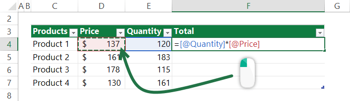
What is on-the-fly formula editing with the mouse? It’s an easy way to select the given parameter of the formula. To add an argument to a function, choose the range of the table using the mouse.
Excel has a built-in autocomplete function; please check the result in the picture below.
In the example, select the Price column and click Enter.
Absolute and relative references
It is good to know that references to single columns in a table are relative by default.
What does it mean? For example, the column references will change when you copy formulas across columns.
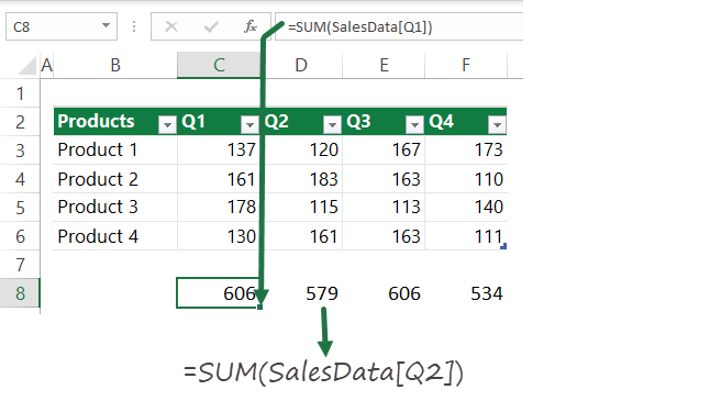
The formula in cell D8 is:
=SUM(SalesData[Q2])in cell E8 is =SUM(SalesData[Q3]) and so on.
As we mentioned in the example above, structured references to multiple columns are absolute. Therefore, the reference will not change if you copy the formula.
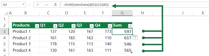
The formula:
=SalesData[@[Q1]:[Q4]]Wrapping things up
Finally, here is a list of what you should know about structured references!
- No special syntax is required to create a formula
- Header or table name changes don’t break the formula
- You can use formulas inside and outside the table
- Supports calculated fields, Excel uses autofill the formulas
Recommended articles