
In this tutorial, you will learn how to Freeze Panes to lock specific cells, rows, and columns in place. If you are working with large data tables, this function is yours! When your spreadsheets become beyond control, you should have to freeze the rows and columns.
Table of Contents:
- Introducing the Freeze Panes feature in Excel
- How to freeze rows
- How to freeze columns
- How to Freeze columns and rows at the same time
Introducing the Freeze Panes feature
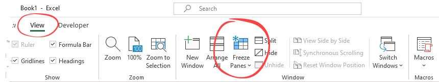
First, just a few words about the Freeze Panes tool. It is one of the most wanted time-saving features in Excel. Locate the ribbon! Find the Window group on the View Tab.
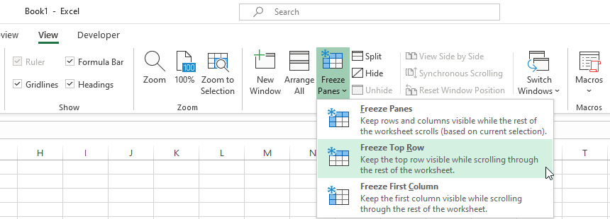
You have three options if you are using the drop-down list.
- The Freeze Panes option can freeze a portion of the data to keep it visible while you scroll through the rest of the main Worksheet.
- If you want to keep only the top row visible while you scroll down, use the Freeze Top Row feature.
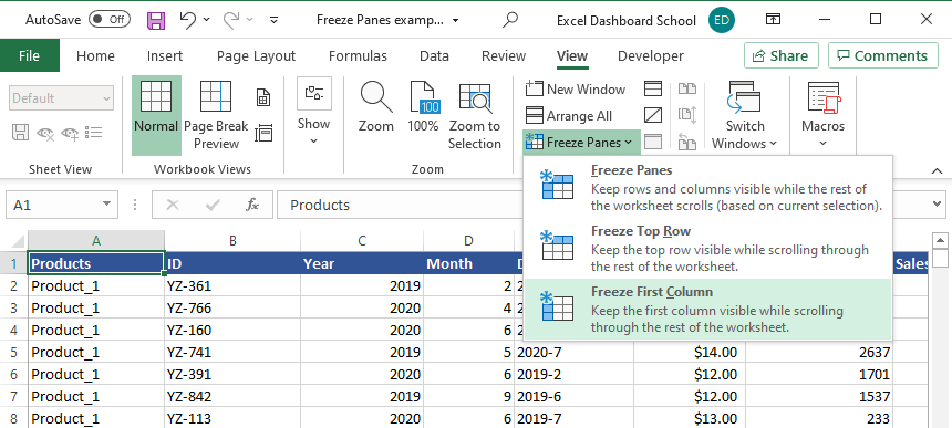
- Keep the first column visible using the Freeze First Column command.
How to Freeze Rows
In this section, you will learn how to freeze a row (or rows) of a worksheet while you scroll to another area of the worksheet.
How to freeze the top row
Let us see how this feature works!
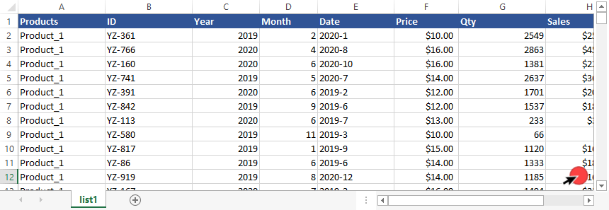
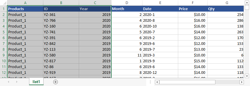
In the example, we have four products in a few regions. The list contains the sales by month from Jan. 2019 to Dec. 2020. The practice file contains 400 rows and 7 columns with different headers.
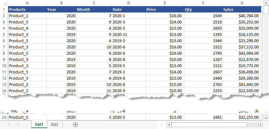
Try to scroll down; for example, jump to cell A122. Houston, we have a problem. The main header will disappear, and the table looks not the best. How to keep the table headers in mind? What should we do?
We will show you how to freeze the header row in place with a few clicks.
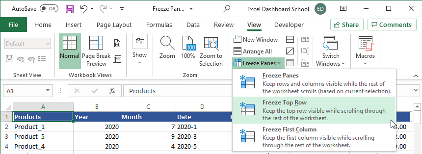
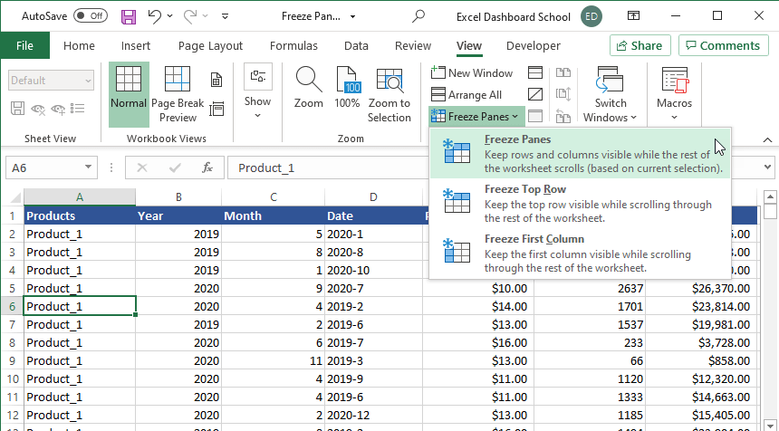
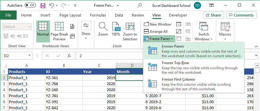
1. Select the row you want to freeze, in this case, row 1.
2. Click the View tab on the ribbon
3. Now, choose the Freeze Panes command and pick the Freeze Panes option from the menu.
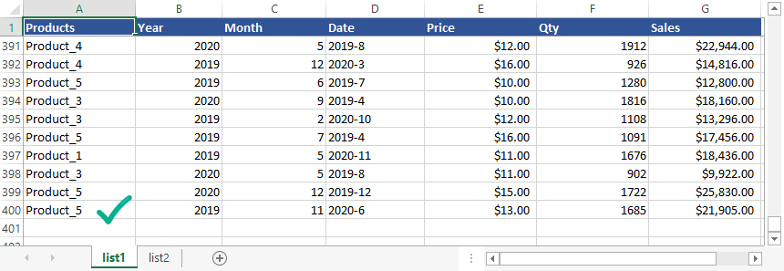
You can check the result in the picture below. The main header remains visible even if you are scrolling the list down.
How to freeze multiple rows (top x rows)
In the next example, you want to freeze the top 5 rows to make a quick comparison. Let us see the steps!
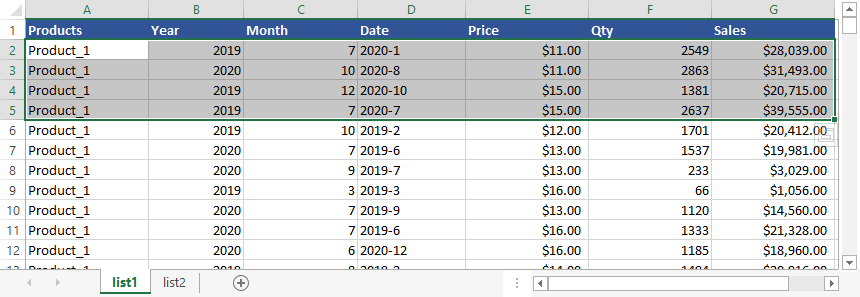
To keep the selected range fixed, go to the next cell in a column, and apply the Freeze Panes command using a drop-down menu.
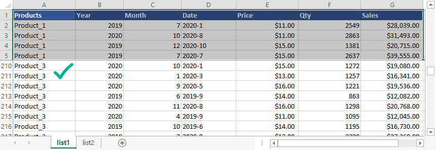
That’s it. The rows will be frozen in place! You will see a gray line; it is a “divider”.
Tip: How to unlock the locked area? To unfreeze a top row or rows, click the Freeze Panes command, then use Unfreeze Panes from the drop-down menu.
How to freeze columns
This guide will give you a quick overview of how to freeze the first (or multiple) columns in Excel.
How to freeze the first column
How to fix your worksheet if a part of your data is out of your viewport? The Freeze First Column command will keep the leftmost column visible when you scroll from left to right or vice versa.
Here is an example:
Okay, try to move the table from left to right using the slider. The Worksheet looks bad! Where is column A? You have not seen the first column, but you must keep the full range visible while you scroll to the right.
You need to fix it. It’s easy!
Select the Freeze First Column in the drop-down menu.
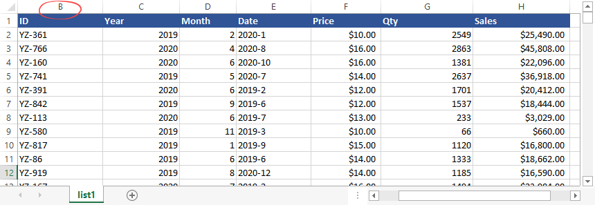
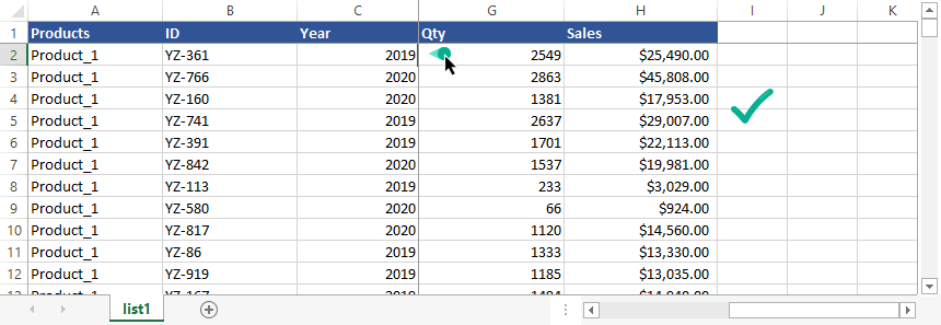
Yes, it works fine! Now you can scroll to the right and back to the left; the main region will remain. That is what you need.
Move the slider at the end of your table, and you will see: the first column is visible.
How to freeze more than one column
Let’s talk about a special case! Let’s say you want to remain in view, not just the first column. In the example, you will learn how to freeze the first three columns.
Like this:
To do that, select a cell in Column D and use the Freeze Panes menu command again!
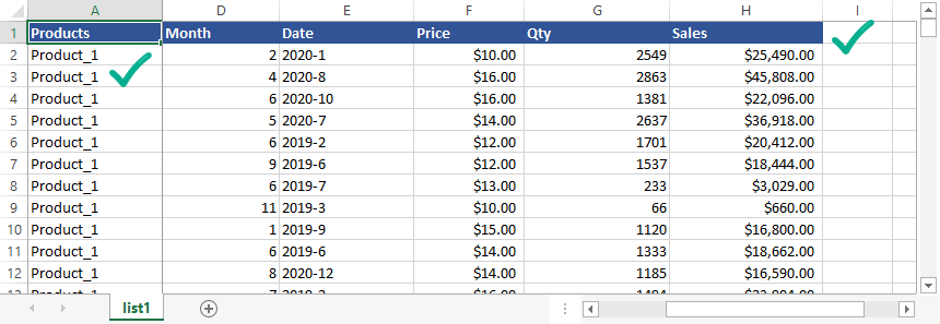
The result looks great. Scroll to the right at the end of the table, and the first three rows remain visible. Quick win!
Freeze columns and rows at the same time
Now you know how to freeze single and multiple rows and columns quickly and easily. It’s time to learn how to freeze columns and rows in sync. How to freeze the first 3 columns and the first 6 rows simultaneously with a single step? Yes, why not?
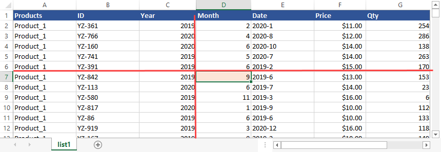
In the example, select cell D7.
The golden rule: The Freeze Panes command will freeze all rows and columns above and to the left. If you want to freeze the first 2 rows and the 3 columns, you should select cell D3!
Additional resources: