
Subscript in Excel is a quick formatting option to decrease the size of a text or a number. Thus, after the operation, the text is smaller.
There are various methods to apply subscript in Excel: apply shortcuts and custom cell formatting, then use the subscript checkbox.
Good news: The shortcut is not short in this case, but much faster than other ways.
How to use the Subscript Shortcut
The subscript shortcut in Excel is Ctrl + 1, Alt + B, Enter
Windows Shortcut
then
Mac Shortcut
then
use the subscript checkbox.
Steps to apply the subscript format:
- Select one or more characters that you want to apply the subscript format. Make sure that you highlight the character(s)
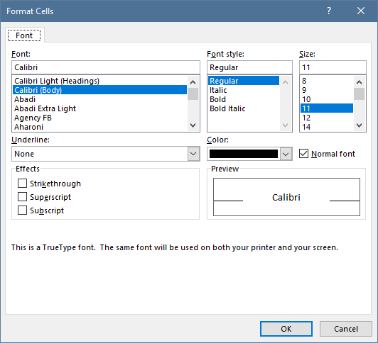
- Use the Ctrl + 1 shortcut to open the Format Cells dialog box
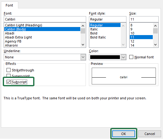
- While the dialog box appears, press Alt+B to mark the Subscript option checked. Press Enter to apply the shortcut.
If you are working on Mac, use the steps below:
- Click on the Formula bar and select the character you want to apply the superscript format
- Press Command + 1 to display the Format Cells dialog
- Under the Effects Group, click the checkbox for subscript, and click OK
Excel Subscript Examples
If you want to use other ways to apply subscript in Excel, you can do that. Let’s see the possible workarounds.
Add a Subscript Shortcut Macro
We always support the faster way to solve a problem. In the first example, we’ll show you how to use a short macro to apply the subscript shortcut effectively.
The macro will use a parameter – str – (you can add it using an input box) to calculate the given position for the format.
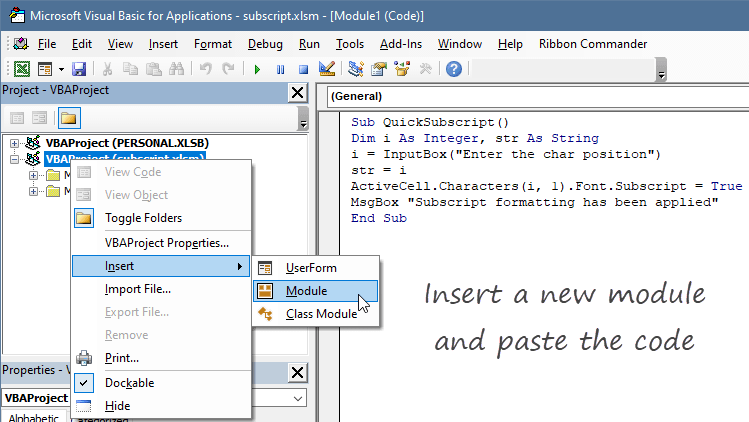
Sub QuickSubscript()
Dim i As Integer, str As String
i = InputBox("Enter the char position")
str = i
ActiveCell.Characters(i, 1).Font.Subscript = True
MsgBox "Subscript formatting has been applied"
End Sub
Now, we’ll explain how to insert the new code.
1. Press Alt + F11 to enter the VBE (Visual Basic Editor)
2. Right-click on the Workbook and choose ‘Insert new module.‘
3. Paste the code, then save the Workbook to a macro-enabled format, like .xlsx or xlsb.
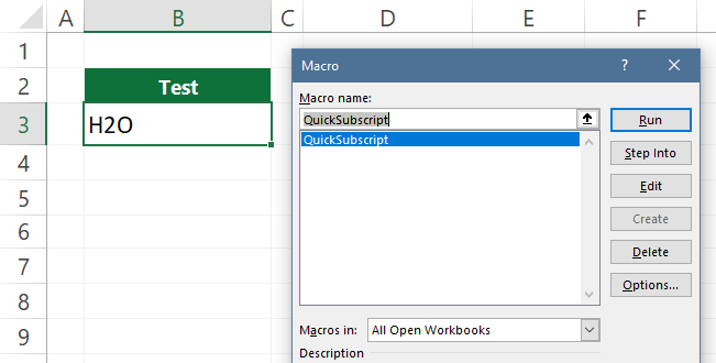
To run the macro, click on the Developer Tab and select macros. Pick our new macro from the list, then run it!
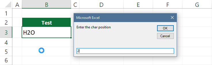
Enter a value (number) where you want to apply the subscript format.
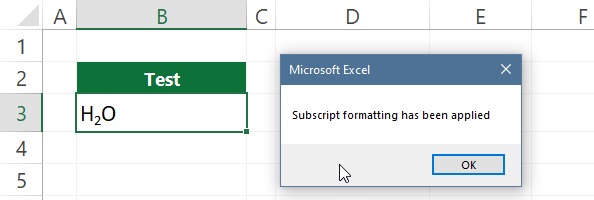
Click OK to apply the subscript on the selected cell.
Example 1: Cell Edit mode
The first method to apply a subscript in Excel is to switch Excel into the cell edit mode using the Edit cell shortcut, F2.
Here are the steps below:
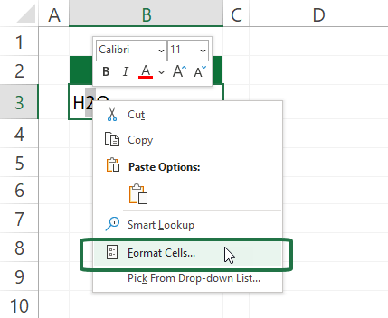
- Double-click or press F2 to edit cell
- Select the character; Excel will highlight it
- Click on Format cells
4. The Format Cells dialog box appears
5. Select the Subscript checkbox under the Effects Group. Next, click OK.
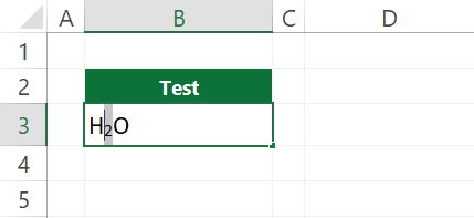
The result is the same as the previous example. Excel will apply the formatting on the second character of the text.
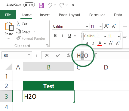
Example 2: Apply formatting using the Formula Bar
You can apply the formatting by editing the text using the Formula Bar.
Let’s see the steps!
1. Select the cell that contains text, then click on the Formula Bar
2. Select the character that you want to format
3. Right-click to open the Format Cells dialog box.
4. Make sure the subscript checkbox is active, then close the dialog box by clicking OK.
Recommended articles
Thank you for reading our guide on how to use subscript in Excel. We recommend you use shortcuts for time-saving purposes. If you are interested, here is a list of our related articles: