
Learn how to extract unique values from a range by using one or more criteria combined with the UNIQUE function and FILTER functions.
Formula to extract unique values with criteria
In the example, you want to extract unique values from the list where the score is greater than 50.
The formula is the following:
=UNIQUE(FILTER(B3:C11, C3:C11>50))
If you are working with complex formulas, it is worth evaluating the expression from the inside out.
=C3:C11>50
This expression returns an array that contains TRUE and FALSE values. For example, look at column E. If the given value in the range meets the criteria, the result is TRUE.
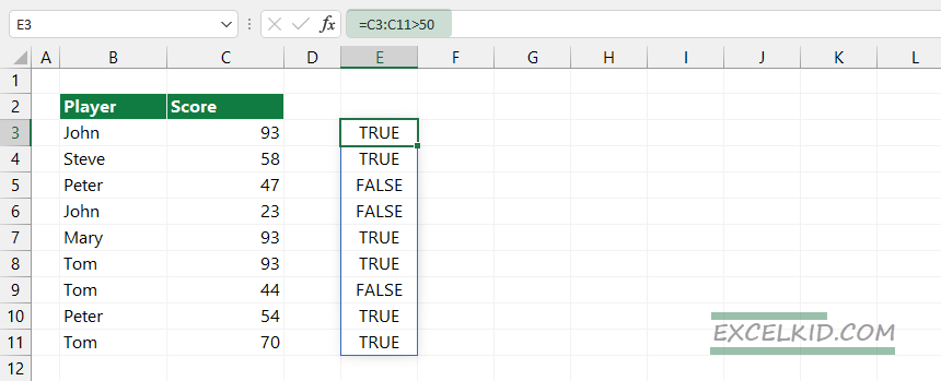
Before we apply the FILTER function, the array looks like this:
- {TRUE, TRUE, FALSE, FALSE, TRUE, TRUE, FALSE, TRUE, TRUE}
- {John, Steve, Peter, John, Mary, Tom, Tom, Peter, Tom}
We will use the result array as a second argument of the FILTER function. The first argument is range B3:B11.
=FILTER(B3:B11, C3:C11>50)
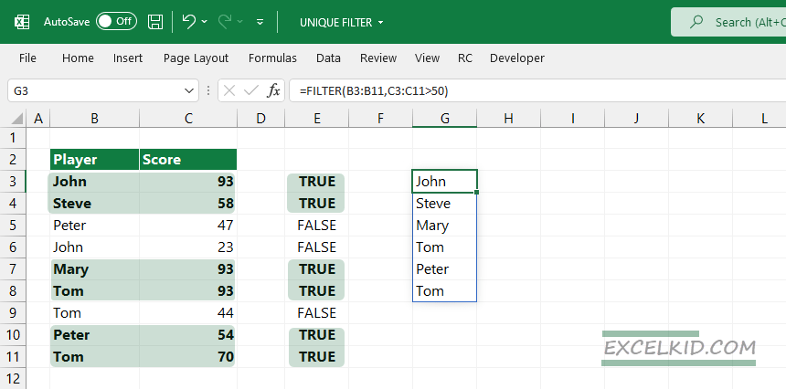
The result_array contains the following names:
{John, Steve, Mary, Tom, Peter, Tom}
The array has six records. As the last step, we will combine the UNIQUE function with the FILTER function to extract unique values:
=UNIQUE(FILTER(B3:B11,C3:C11>50))
Result:
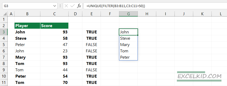
The result is an array of five records.
Extract values with multiple criteria
Here is a detailed example if you need to use multiple criteria. In this part of the tutorial, we will show you how to extract unique values from a list based on multiple logical criteria. Using the UNIQUE and FILTER function together is a great idea if you want to filter and reduce your data set.
Generic formula:
=UNIQUE(FILTER(data,(logical_test) * (logical_test)))
The formula uses two steps to extract the values that are met two logical criteria. First, the FILTER function removes data that does not meet the required criteria. After that, the UNIQUE function reduces results and shows only unique values.
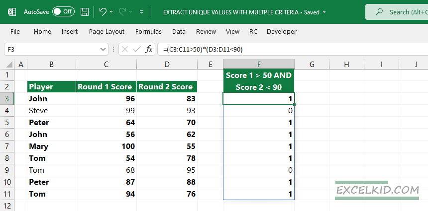
In the example, we will combine two logical tests in an expression. The FILTER function returns an array where Score 1 > 50 and Score 2 < 90.
Evaluate the expression below:
=(C3:C11>50)*(D3:D11<90)
The result is an array: {1, 0, 1, 1, 1, 1, 0, 1, 1}
The FILTER function will use the array as an argument. If the value is TRUE, the function will return the correspondent record.
Formula:
=FILTER(B3:B11,(C3:C11>50)*(D3:D11<90))
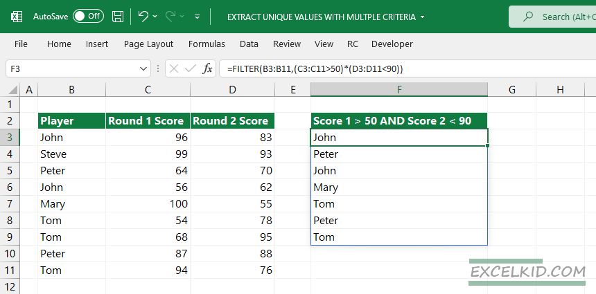
Note: The array contains TRUE and FALSE values that follow the Boolean logic.
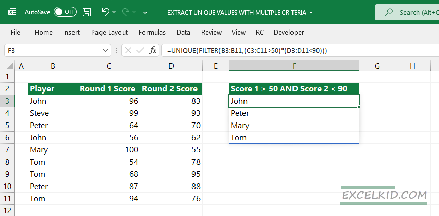
Finally, apply the UNIQUE function to extract unique values.
=UNIQUE(FILTER(B3:B11,(C3:C11>50)*(D3:D11<90)))
Additional resources
- Excel Formulas
- Count unique text values
- How to remove duplicates in Excel