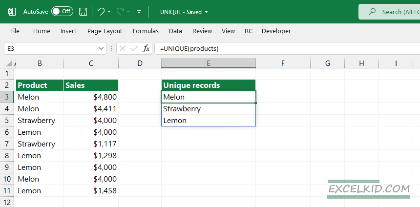
The Excel UNIQUE function extracts unique values from a range and returns a list of unique values in a list or range.
In a nutshell, The UNIQUE function can handle various data types. For example, you can use text, numbers, and date values and return an array of unique values. The function is available for Microsoft 365 users.
Syntax and Arguments of the UNIQUE function
Here is a UNIQUE function’s syntax.
=UNIQUE (array, [by_col], [exactly_once])
Arguments:
- array is the range or array from which to return unique rows or columns.
- by_col is a logical value. It controls how to compare and extract values. FALSE is the default value and extract values by row. In the case of TRUE, the function extracts values by column.
- exactly_once is a logical value. If the value is FALSE, the function extracts all distinct values. If the argument is TRUE, the function extracts values that occur exactly once. The default value is FALSE.
How to use the Excel UNIQUE function
The UNIQUE function evaluates an array and extracts the unique values to another array. The result is a dynamic array that contains a list of unique values.
UNIQUE is a member of dynamic array functions in Excel. Therefore, formulas that return multiple values spill these values directly onto the worksheet. You will get the result as an array. Excel will update the result array if you add or remove values to a source range.
The function uses three arguments. The ‘array’ is required. The ‘by_col’ and ‘exactly_once’ are optional.
Examples
In this section, we will demonstrate how the function works through easy-to-understand examples.
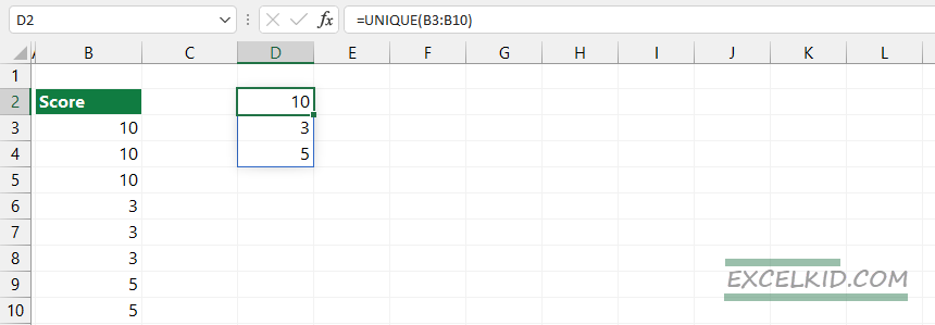
Basic usage of the UNIQUE function
In the example, we want to extract unique values from the range B3:B10. Use the formula without the second and third arguments:
=UNIQUE(B3:B10)
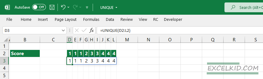
Using the ‘By column’ argument
As we mentioned above, the UNIQUE function extracts unique values in rows by default.
If you use UNIQUE without the second argument, the function can not handle the values in columns.
Formula:
=UNIQUE(D2:D12)
In the following example, we will add TRUE as a second argument; the function will handle the horizontal array properly.
Formula:
=UNIQUE(D2:D12, TRUE)
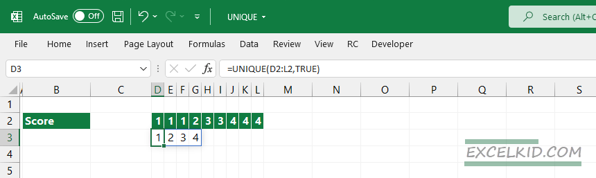
The returned array contains unique values only.
Using the ‘exactly once’ argument
Take a closer look at the differences between “distinct” and “exactly once”.
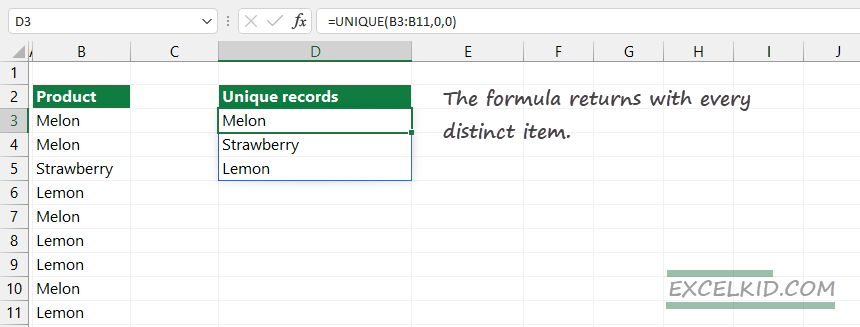
As we stated above, the third argument is optional. The “exactly_once” decides how the function handles duplicated values. By default, it uses FALSE and returns with every distinct item:
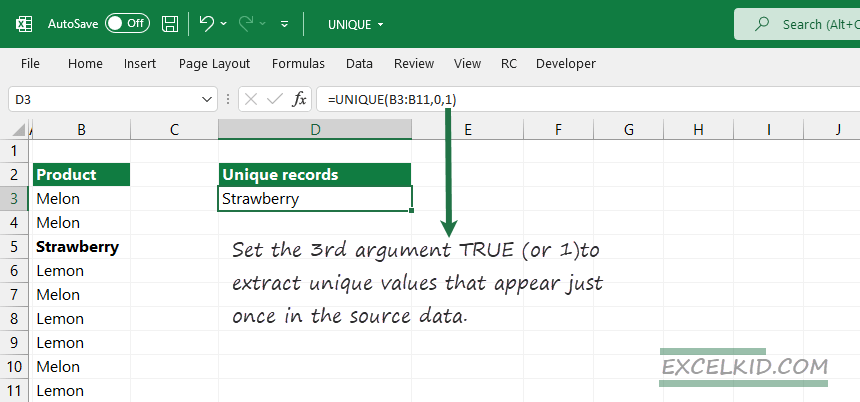
Apply TRUE (or 1) for exactly_once argument. The function returns unique values that appear exactly once in the source range.
Both formulas below return the same result:
- =UNIQUE(B3:B11,0,1)
- =UNIQUE(B3:B11,,TRUE)
Now, we have learned almost all about the UNIQUE function.
Workaround with criteria
Working with Excel, you may need to extract unique values based on a logical test. Learn how to use the FILTER and UNIQUE functions in one formula.
Generic formula to use a criteria:
=UNIQUE(FILTER(range1, range2 = B1))
If you want to learn more about this formula, you can find our detailed guide here.
Additional resources