Learn how to sum every nth row (for example, every second, third, or fifth row) in Excel using the SUMN or SUMPRODUCT function.
How to sum every nth row
- Type =SUMN(B3:B10, 2)
- Press Enter
- The formula returns the sum of every nth row
The formula uses the following syntax:
=SUMN(range, nth, optional [startAtBeginning])There are two required and one optional argument.
Example
In the example, the goal is to sum every second row. To create a formula, first, configure the SUMN function arguments:
- Range = C3:C12
- Nth = 2
Formula:
=SUMN(C3:C12,2)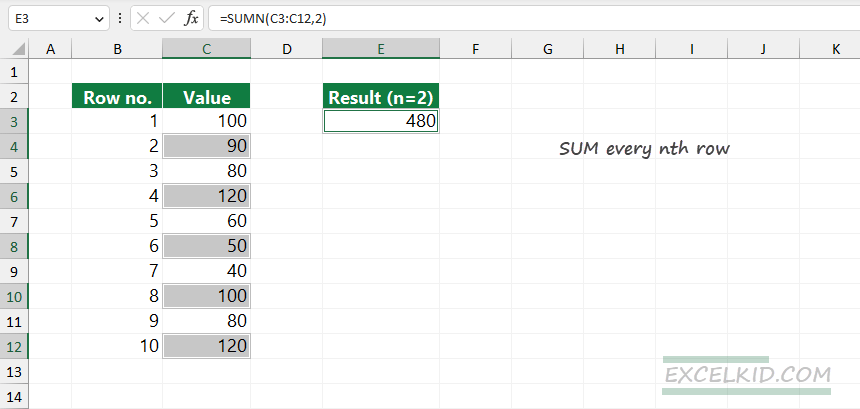
The formula creates an array that contains the following values:
={90, 120, 50, 100, 120}Next, SUMN sums the numbers in the array and returns 480.
Note: If you want to sum every nth row starting with the first row, set the 3rd argument to TRUE. In this case, the formula will return the sum of the 1st, 3rd, 5th, 7th, and 9th rows.
What if the given row contains more than one value? Modify the first argument (append the selection to C3:D12), and the formula will work fine.
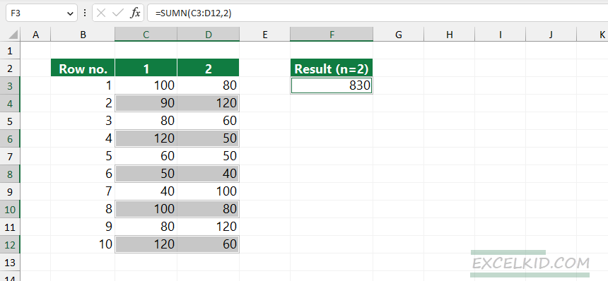
Formula:
=SUMN(C3:D12,2)The SUMN function is a part of our UDF add-in.
Sum every nth row using MOD and ROW functions
To summarize every nth row, you can use a formula with SUMPRODUCT, MOD, and ROW functions.
Generic formula:
=SUMPRODUCT(--(MOD(ROW(row_numbers)-ROW(B3)+1,nth_value)=0), values)We use a named range, “rnum” which refers to range B3:B12, and “values,” which refers to range D3:D12.
In this case, the formula in cell G4:
=SUMPRODUCT(--(MOD(ROW(rnum)-ROW(B3)+1,2)=0), values)Now, evaluate the formula from the inside out. The ROW function gets a set of row numbers for the range, which looks like this:
= {3, 4, 5, 6, 7, 8, 9, 10, 11, 12}The array starts with 3 since the row reference is 3. After that, the MOD function returns the remainder for each row number divided by N.
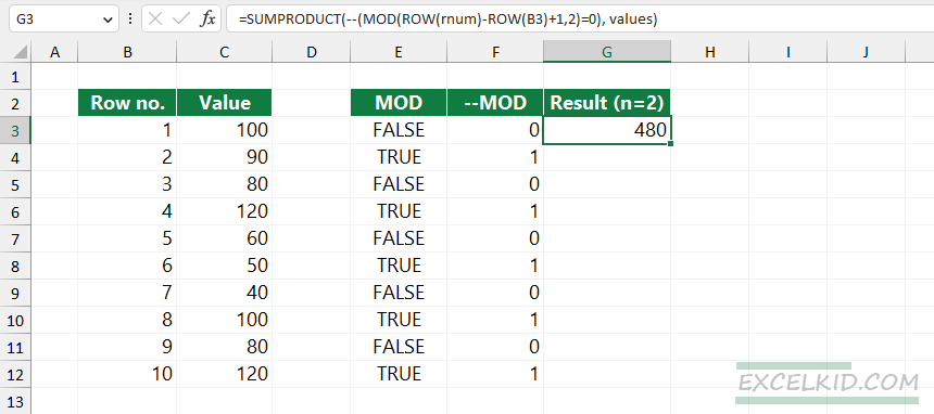
The MOD function returns an array that contains Boolean values, so we need to use the double negative method to convert TRUE and FALSE values to 0s and 1s.
The output array looks like the following:
={0,1,0,1,0,1,0,1,0,1,0,1}In the example, nth=2, the MOD function will return the array below. Where the value equals 1, SUMPRODUCT multiplies and then sums all values in the array. In the example, the total for every second row is:
=(90 + 120 + 50 + 100 + 120) = 480This method works fine when you want to sum every nth column; you can replace the ROW function with COLUMN.