
This definitive guide will show you how to apply the Excel strikethrough shortcut as a checkmark alternative using five methods.
Let’s talk about the point before diving deep into the details and examples.
What is Strikethrough in Excel?
Strikethrough is a cell-related feature in Excel. This function crosses the cell content (text or numbers) by drawing a vertical line.
If you want to practice, download this Strikethrough Shortcuts Excel Template here.
Effective Ways to use Strikethrough in Excel
First, we will introduce the most common ways of Using Strikethrough Shortcut in Excel:
- Use the Excel Strikethrough Shortcut Key
- Apply the Format Cells Options
- Use the Quick Access Toolbar (QAT)
- Add a Strikethrough Tab to the Excel Ribbon
- Use Conditional Formatting Formulas
- Write a small VBA code to apply Strikethrough in Excel
#1 – Use the Excel Strikethrough Shortcut Key
Steps to apply strikethrough in Excel using a keyboard shortcut:
- Select the source cells in which you want to apply the strikethrough formatting style.
- Apply the Ctrl + 5 Excel strikethrough shortcut key
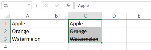
Windows shortcut
Mac shortcut
#2 – Apply the Format Cells Options
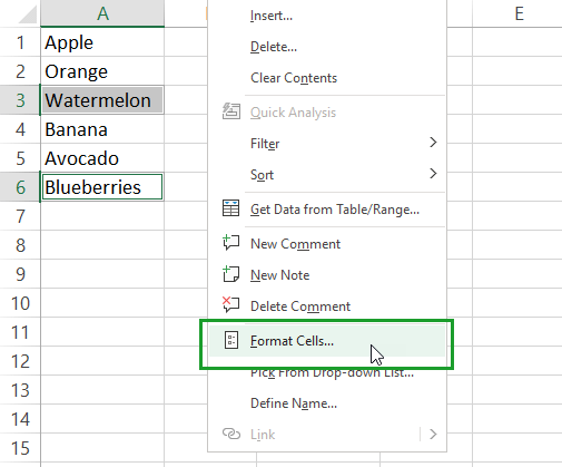
If you don’t know how the strikethrough shortcuts work, there are further options for you to add a strikethrough to cell content.
Step 1. Right-click on the selected cells and choose the Format Cells option from the context menu.
Step 2: Locate the Font Tab on the ribbon and select the “Strikethrough” option. Finally, click OK.
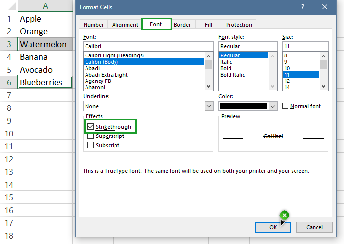
Result: The cell is strikethrough formatted.
#3 – Use the Quick Access Toolbar (QAT) to apply strikethrough
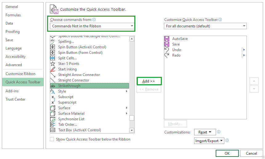
Good to know that this option is not available in the Quick Access Toolbar by default. So, you need to add it to the QAT.
Step 1: Go to the ribbon and select the ‘Customize Quick Access Toolbar‘ by right-clicking the Tab name.

Step 2: Select the “Choose commands from” option, use the drop-down list, and pick the ‘Commands not in the Ribbon’ from the list.
Step 3: Scroll down and find the Strikethrough command. Highlight the command and click ‘Add.’ Now, the option is available on the QAT and ready to use.
The strikethrough shortcut is now available on the QAT.
Step 4: Select the cell or range of cells to which you want to apply strikethrough. Finally, click on the Strikethrough icon.
The command will Strike the selected cells through.
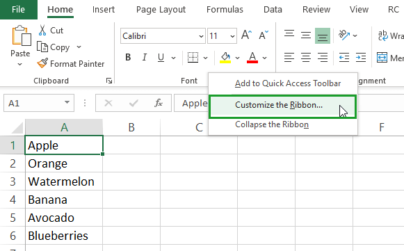
#4 – Add a Strikethrough Tab to the Excel Ribbon
If you prefer using the ribbon, this section is yours.
Step 1: Select the Home Tab and locate the Font Group. Right-click on the group and select the ‘Customize the ribbon’ command.
Step 2: Jump to the customization area, which you can find at the bottom-right section of the window.
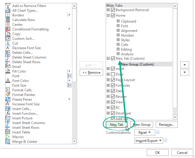
Step 3: Choose a strikethrough command from the right-side list and click Add. Click Add “New Tab,” Finally, choose the “Strikethrough” option, then press OK.

Step 4: Click OK to close this window and look at the ribbon. A new tab appears on the ribbon, and you can reach the strikethrough shortcut quickly.
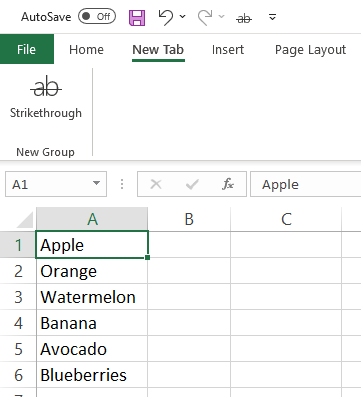
Tip: We recommend the example above if you want to collect your favorite functions into a single Tab.
#5 – Use Conditional Formatting Formulas
If you prefer using conditional formatting and formulas, we have good news. Using dynamic formulas – based on formatting rules – you can apply Strikethrough in Excel.
Step 1: Select the cell or range where you want to apply the strikethrough formatting.
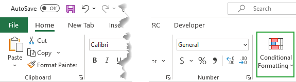
Step 2: Select the Home Tab and click Conditional Formatting.
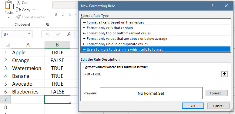
Step 3: Add a new Formatting rule
Step 4: Choose the ‘Use a formula to determine which cells to format’ command.
Step 5: Enter the formula, in this case, B1 = TRUE, but don’t click OK
Step 6: Select Format
Step 7: On the Font Tab under the Effects group, select strikethrough
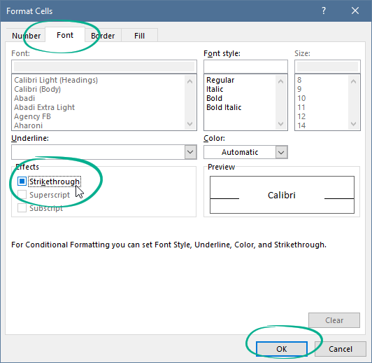
Step 8: Click OK
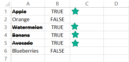
If the rule is true (the cell value = TRUE), conditional formatting will apply the strikethrough format.
Tip: If you manage multiple tasks using your project management template, use conditional formatting formulas and a simple drop-down list. In Column B, change the value from ‘No’ to ‘Yes’ when you close a task or milestone.
#6 – Write a small VBA code to apply Strikethrough in Excel
Here are two useful examples using Visual Basic for Applications (VBA)
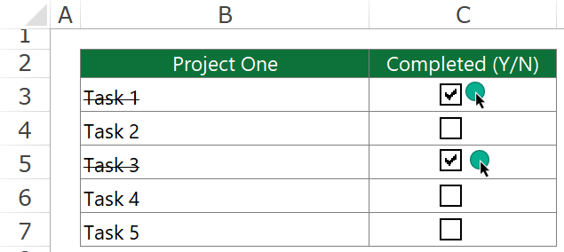
Example 1: Replace the Strikethrough shortcut using checkboxes
We like Excel Form Controls, so let us see an excellent example using checkboxes.
Just click on the given checkbox, and Excel will apply the strikethrough using a single click. Thus, you only need to write a basic macro to speed up your work. Looks great, is not it?
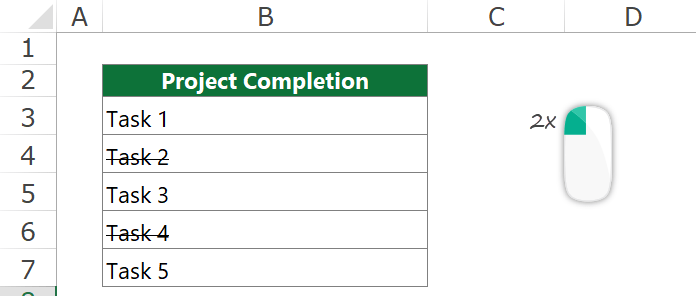
Example 2: Automated Strikethrough format using macros
The double-click event in VBA is the fastest way to apply the strikethrough in a cell.
How does it work?
This method disables the cell edit mode in Excel. Use a double click over the cell, and the event will apply the strikethrough format on the spot.
Frequently Asked Questions – Final Thoughts
No, it works if the cell has content. The function is useless if you have blank cells.
No, it does not change the cell value. So, for example, “ABC” is the same as “ABC” for all Excel formulas.
You can use the Ctrl + Z keyboard shortcut to undo the command. Furthermore, repeat the abovementioned methods, like an on-off switch.
Yes, it is possible. First, edit the cell (highlight the text) and select the part of a cell that you want to format.
If we use conditional formatting for strikethrough, use relative references instead of absolute ones.
Recommended Articles
Thanks for being us today, and read our ultimate guide about Strikethrough Shortcuts in Excel. Here is some related tutorial: