
The Excel HLOOKUP function searches for a certain value in a row and returns a value from a different row in the same column.
Tip: If you are using Excel for Microsoft 365, try the XLOOKUP function, an improved version of Excel lookup functions that work in any direction and returns exact matches by default without optional arguments.
How to use the HLOOKUP function in Excel?
Use HLOOKUP if your table array is transposed (variables headers listed in a row). The HLOOKUP function searches for a given lookup value in the first row of a table. When it finds a match, the function returns a value from the row shown in that column. HLOOKUP function supports wildcards to find partial matches.
First, take a look at the syntax and function arguments.
Syntax:
The HLOOKUP function uses three required and one optional argument.
=HLOOKUP(lookup_value, table_array, row_index, [range_lookup]
Arguments
- lookup_value is the value that you want to look up;
- table_array is the range from which you want to find and retrieve data
- row_index is the row number containing the return value
- range_lookup is FALSE (or 0) for an exact match. Use TRUE (or 1) for an approximate match. The default value is TRUE.
HLOOKUP Function Examples
In this section, we will demonstrate HLOOKUP examples.
Example #1 – Exact match
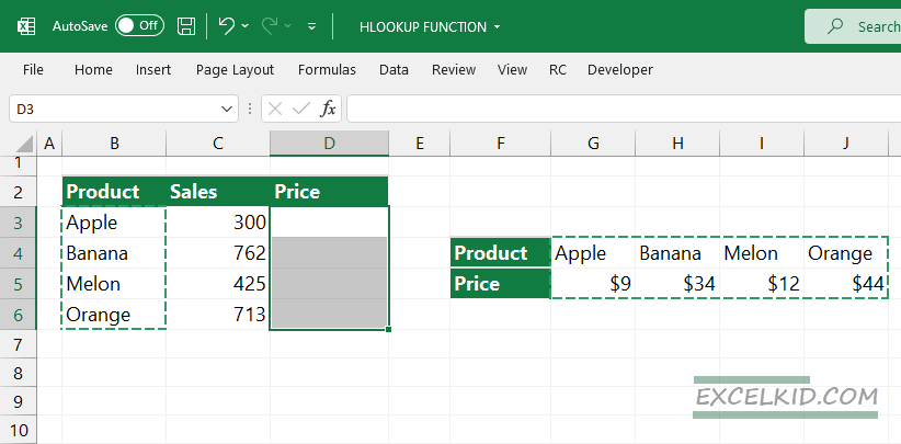
With an HLOOKUP function, we search the product name in the data table and return the value from the second (Price) row.
Create a named range first! Select the table array. This range is where you are looking for the lookup value. In this case, select range G4:J5. Locate the name box and type ‘data‘.
From now, the range G4:J5 refers to ‘data’.
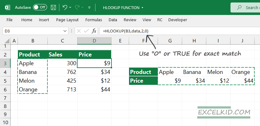
Type the formula below in D3:
=HLOOKUP(B3,data,2,0)
- B3 is the lookup value (Apple) that we are trying to match in the table array (data).
- Table array is the second argument; in this case, use the named range ‘data’, to simplify the formula
- The row index is 2. This row contains the return value we are looking for
- We find an exact match, so use the ‘0’ (or FALSE) logical value as the 4th, optional argument
Result:
Example #2 – Approximate Match
Sometimes, we need to use an approximate match instead of an exact match. In the example, we want to create categories based on sales. Therefore, the lookup value is “A” in cell C3.
The ‘data‘ named range is the same as we mentioned in the first example: G4:J5
Now change the 4th argument to TRUE (or 1):
=HLOOKUP(C3,data,2,1)
or use the function with the required three arguments only:
=HLOOKUP(C3,data,2)
Here is the result if you are using an approximate match:
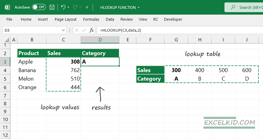
The lookup value is 308, and the range_lookup argument is TRUE. Excel evaluates the formula, and no exact match is found.
In this case, the HLOOKUP function gets the nearest value (300) that is less than the lookup value and returns with “A”.
HLOOKUP Function: range lookup argument
It’s time to summarize what we have learned about the range_lookup optional argument:
- The range_lookup helps you decide: are you trying to match an exact lookup value TRUE or something similar FALSE. The default value is TRUE, which allows a non-exact match.
- Apply the FALSE value if you need to require an exact match.
- If range_lookup is TRUE, and HLOOKUP does not find an exact match, the function will return the largest value that is less than the lookup value.
- HLOOKUP returns an exact value if one exists, even if you use TRUE as the last argument.
- If range_lookup is TRUE, you must sort the lookup values in the first row of the table in ascending order. Otherwise, HLOOKUP may return an unexpected value.
- In the case of the FALSE argument, it is not necessary to sort the table.
Additional resources