Filter Shortcut

Discover the most wanted Excel filter shortcut list! Apply or remove filtering and sort your data through useful examples.

How to Filter Data using Keyboard Shortcuts

If you work with lists or a table, you can apply filter shortcuts or move the mouse over the table header row and filter like a drop-down list.

This article will explain how to use shortcuts for filtering and displaying data in Excel.

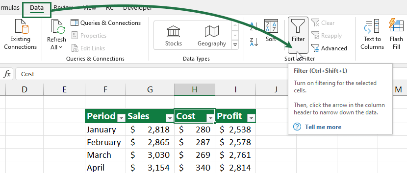
1. Turn filtering on or off

Select a cell in a range and use the Ctrl + Shift + L keyboard shortcut.

Tip: Convert the range to an Excel table using the Ctrl + T insert table shortcut, and the filter will appear automatically.

Another way to activate the filter:

Select the Data tab. Under the Sort & Filter Group, click on the Filter icon.

2. Filter menu

Steps to show the Filter menu in Excel:

1. Select the header row, and locate the column where you want to apply the filter
2. Locate the down arrow
3. Use the Alt + down arrow shortcut to display the Filter menu for the selected column

3. Filter Menu Navigation using arrow keys

Filter menu navigation between options is easy if you use the arrow keys. In the example, you want to apply number filters. First, press the down arrow key to select the Number Filters option. Now press the right arrow key once to navigate to ‘Greater than or equal to‘ logical operator. Finally, press Enter.

4. Remove all filters

In the following example, you have more than one filter. How to remove all?

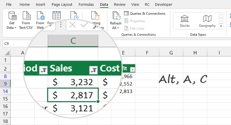
Shortcut to remove all filters:

Alt, A, C

5. Clear filters in a column

Steps to clear the filter in a single column:

1. Select the column header
2. Press Alt + down arrow key
3. The Filter menu appears for the selected column
4. Press C to clear the filter

6. Drop-down menu shortcuts using underlined letters

Excel provides built-in shortcut keys (underlined letters) to apply various filter commands in the Filter menu. To use filter shortcuts in the drop-down menu, press the Alt + down arrow key.

These are the following:

• S – Sort data A to Z
• O – Sort Data Z to A
• T – Sort by Color using the Custom Sort option
• C – Clear all filter
• I – Filter by Color (when available)
• F – Number / Text Filters (it depend on cell value)
• E – Enter a filter value manually (search bar)

For example, type the letter “I” to filter data by color. This option is available only if your range contains color(s).

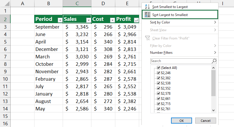
7. Quick Sorting Shortcuts

In Excel, there are various methods for sorting. However, the fastest way is using the following shortcuts:

• Press Alt + down arrow, then ‘S’ to sort your data in ascending order.
• Press Alt + down arrow, then ‘O’ to sort your data in descending order.

There are two options available, and it depends on the type of data you want to sort.

Tip: In the example, we use the Profit columns for sorting purposes. In column E, the data type is number, so you’ll see the ‘sort largest to smallest‘ command. In the case of text data, you’ll see the ‘sort Z to A‘ function.

8. Search box

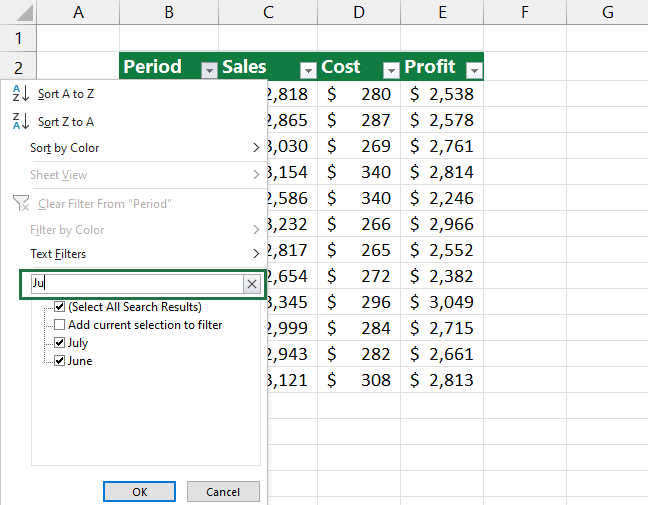
Excel uses the Filter menu Search box to provide custom filter options. In the example, we are working with text data in column B.

Start typing your search criteria, and Excel creates a filter in the selected column.

9. Display the Custom AutoFilter dialog box

Shortcut to open the custom filter dialog box:

1. Select the column in the header where you want to apply the filter
2. Press Alt + down arrow key
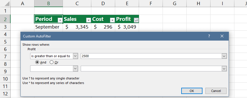
3. Release the keys and press F, then E to display the Custom AutoFilter dialog box

Enter criteria for the Profit column. In this case, we want to show only values greater than or equal to 2500. Click OK to filter the data.

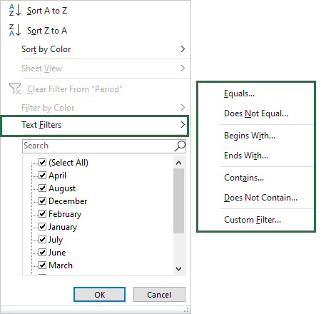
10. Shortcut keys for Text Filters

If you are working with text values, use the following filter shortcuts that you can use after opening the Custom Filter dialog box:

• Equals: Alt + ↓ + F + E
• Does Not equal: Alt + ↓ + F + N
• Begins with: Alt + ↓ + F + I
• Ends with: Alt + ↓ + F + T
• Contains: Alt + ↓ + F + A
• Does not contain: Alt + ↓ + F + D
• Custom Filter: Alt + ↓ + F + E

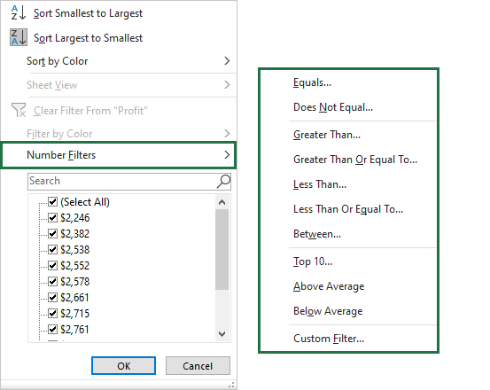
11. Shortcut keys for Number Filters

In the case of numerical values, use these shortcuts after opening the Custom Filter dialog box. I’ll list only the differences to text values:

• Greater Than: Alt + ↓ + F + G
• Greater Than Or Equal To: Alt + ↓ + F + O
• Less Than: Alt + ↓ + F + L
• Less Than Or Equal To: Alt + ↓ + F + Q
• Between: Alt + ↓ + F + W
• Top 10: Alt + ↓ + F + T
• Above Average: Alt + ↓ + F + A
• Below Average: Alt + ↓ + F + B

Final thought

It was our definitive guide on using the filter shortcuts in Excel. Stay tuned.

Additional resources:

• Excel Shortcuts