Count cells between two numbers - Quick Guide

To count cells between two numbers in Excel, you can use the COUNTBETWEEN function or the COUNTIFS function.

How to count cells between two numbers

Here are the steps to count the number of cells between two numeric values in a selected range:

Type =COUNTBETWEEN(B3:B11,100,200)
Select the range (B3:B11) that contains numbers.
Add the lower limit (100).
Add the upper limit (200).
Press Enter.
The function will return the number of cells between the lower and upper limits.

COUNTBETWEEN function

COUNTBETWEEN is a powerful user-defined function. Use it if you want to create easy-to-readable formulas instead of using built-in functions.

Syntax

=COUNTBETWEEN(cRange, lowB, upB, [iLimits])

Arguments

The function uses three required and one optional argument.

cRange is a range of cells that contains numeric values.
lowB is the lower bound
upB is the upper bound
iLimits is an optional argument; it controls that the functions count the lower and upper limits.

Example

In the first example, your data set is in cell B3:B11, and you want to count cells between 3000 and 5000. So first, select the range that contains values, and add a name to a range, for example, “Sales”. From now on, “Sales” refers to the B3:B11 range.

Configure the arguments of the COUNTBETWEEN function:

range = “Sales”
lower limit = 3000
upper limit = 5000

Formula:

=COUNTBETWEEN(Sales, 3000, 5000)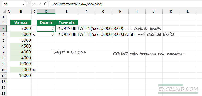

Evaluate the formula. COUNTBETWEEN creates an array that meets the given criteria: the value is greater than or equal to 3000 and less than equal to 3000. Without using the optional iLimit argument, the return array contains the following numbers:

={3000, 4500, 4000, 4000, 5000}

Finally, the formula counts the values in the array. So, the result is 5.

If you want to exclude the lower and upper limits (in other words, you want to apply the “greater than” and “less than” criteria), set the optional argument to FALSE.

Formula:

=COUNTBETWEEN(Sales, 1000, 5000, FALSE) = {4500, 4000, 4000} = 3

The result is 3; the formula does not count the lower and upper limits (3000 and 5000).

Code

Function COUNTBETWEEN(ByVal cRange As Range, _
ByVal lowB As Single, ByVal upB As Single, _
Optional ByVal iLimits As Boolean = True) As Variant

Dim currentCell As Range
Dim count As Integer
count = 0

For Each currentCell In cRange
    If (iLimits = True And currentCell.Value >= lowB And currentCell.Value <= upB) _
    Or (iLimits = False And currentCell.Value > lowB And currentCell.Value < upB) Then
        count = count + 1
    End If
Next currentCell

COUNTBETWEEN = count
End Function

COUNTIFS function to count cells between two numbers

If you are unfamiliar with user-defined functions, you can use the COUNTIFS function to count the number of cells that contain values between two numbers. COUNTIFS uses range/criteria pairs, so it is easy to define the lowest and the highest numbers between the values the function will count.

The general formula is:

=COUNTIFS(range, criteria1, range, criteria2)

In the example, we want to count the number of cells between two numbers. The lower band is 3000; the upper band is 5000. COUNTIFS uses multiple criteria. To include the lower and upper limits, use logical operators and the following conditions:

Criteria1: >= 3000, (“greater than or equal to”)
Criteria2: <= 5000, (“less than or equal to”)

Formula:

=COUNTIFS(Sales,”>=”&3000, Sales,”=<”&5000 = 5

If the given value in the selected range meets both criteria, COUNTIFS will count the cell.

Workaround with SUMPRODUCT

In the SUMPRODUCT-based formula, we will use boolean logic.

Formula:

=SUMPRODUCT((Sales>=3000)*(Sales<=5000))

SUMPRODUCT will return an array with TRUE or FALSE values. We have two criteria, so the result is two arrays:

=Sales>=3000 = {TRUE, TRUE, TRUE, TRUE, TRUE, TRUE, TRUE, TRUE, TRUE}
=Sales<=5000 = {FALSE, TRUE, FALSE, TRUE, TRUE, TRUE, FALSE, TRUE, FALSE}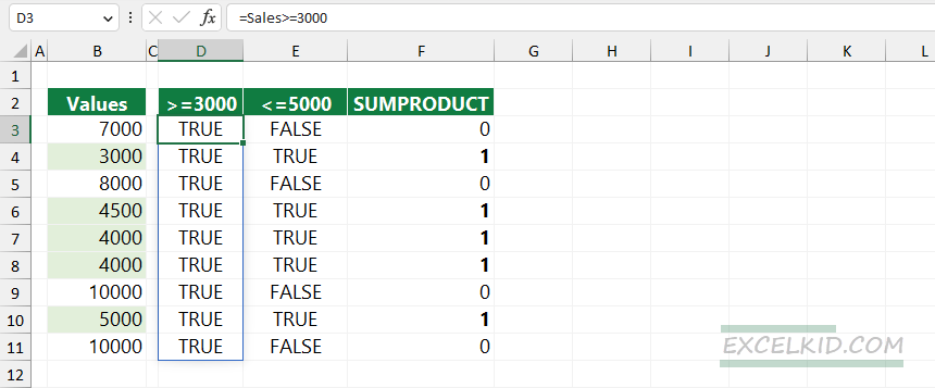

The formula converts boolean TRUE and FALSE values to 0 or 1.

=SUMPRODUCT({0,1,0,1,1,1,0,1,0}) = 5

If the value meets both criteria, the result is 1. SUMPRODUCT will return the sum of the numbers in the array, 4.

Additional resources and related formulas