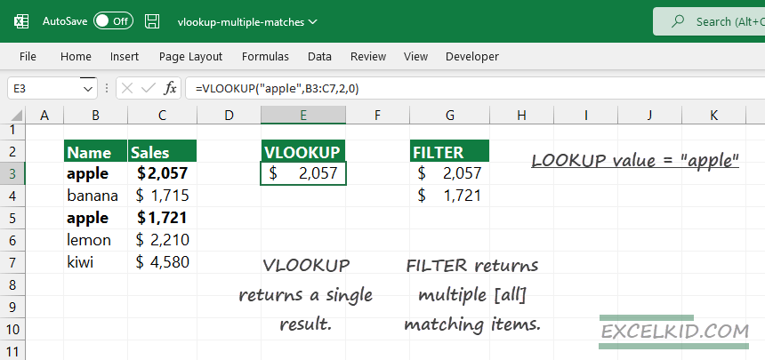
Today’s guide will show how to return and display multiple matches using the VLOOKUP function or apply the FILTER function.
VLOOKUP returns a single result by default. So, to display multiple results, you must apply some workarounds using custom formulas. We will show you various methods to perform the task.
How do I get VLOOKUP to return multiple matches?
- Apply the FILTER function
- Use the array argument that contains the possible matches
- Set the include argument to lookup_array = lookup_value
- The formula returns multiple matches
Here is the formula to get all matches using the FILTER function:
=FILTER(C3:C7, B3:B7=”apple”)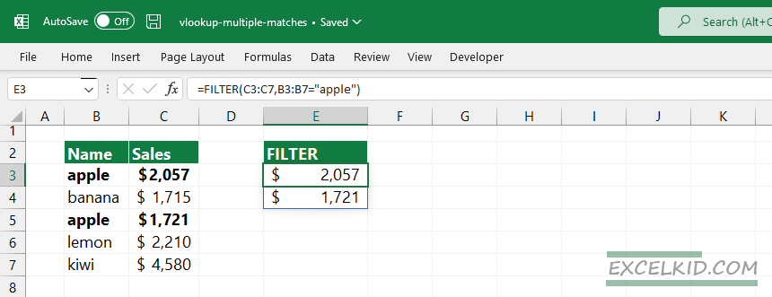
The first argument [array] contains the lookup value “apple”. The second argument, [include], will find and extract multiple matches from the Sales column.
How to use VLOOKUP with multiple results
If you want to use VLOOKUP for multiple matches, it is necessary to apply a little trick.
Because the FILTER function is available in Excel 2019 and above, we will show you the solution if you have an older Excel version.
First, we will insert an additional column (helper column) into the data table. With the help of the COUNTIF function, it’s easy to create a unique identifier for all matching results. The helper column uses the COUNTIF function to create a unique ID for each instance.
Take a closer look at the formula in cell F2:
=B3&COUNTIF(B3:B$7,B3)To create a unique name for all instances, we need to merge the original lookup value using an ampersand character. This is why we leave the B3 part of the expression unlocked. Copy the formula down!

In column B, we have multiple matches in the case of “apple”. Using the COUNTIF function, the formula will create a list in column F that contains unique names. VLOOKUP function will use the unique records as the first argument (lookup value) of the VLOOKUP function.
Let us see the next step!
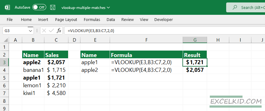
Replace the original range with values that do not contain duplicate values. The new data set is located in range B3:B7. To get multiple matches using VLOOKUP, apply the following formulas to get the sales where the product name is “apple”:
=VLOOKUP(E3, B3:C7,2,0) = $1721
=VLOOKUP(E4, B3:C7,2,0) = $2057
Get Multiple Matches using INDEX and MATCH
The following workaround uses the INDEX, MATCH, and INDIRECT functions to return all matches based on a lookup value.
Note: if you are working with array formulas, you must simultaneously press the Ctrl + Shift + Enter keys, then release all keys. You will see curly brackets around the formula.
Formula:
={INDEX($C$3:$C$7, SMALL(IF(ISNUMBER(MATCH($B$3:$B$7,$E$3,0)), MATCH(ROW($B$3:$B$7), ROW($B$3:$B$7)),""), ROWS($A$1:A1)))}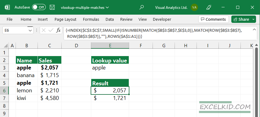
Explanation
The MATCH function returns an array. In case of a match, the function returns with 1. Else, we get #N/A.
=MATCH($B$3:$B$7,$E$3,0)
={1,#N/A,1, #N/A, #N/A }
We use the ISNUMBER function to convert the numeric values to boolean values:
=ISNUMBER(MATCH($B$3:$B$7,$E$3,0))
={TRUE, FALSE, TRUE, FALSE, FALSE}
The next step is to convert boolean values to row numbers and blanks using the IF function. For example, use the MATCH and ROW functions to create a sequential order from 1 to n. The formula returns an array that contains the positions of the matching values in column D.
=IF(ISNUMBER(MATCH($B$3:$B$7, $E$3, 0)), MATCH(ROW($B$3:$B$7), ROW($B$3:$B$7)), "")Result:
={1, "" ,3, "", ""}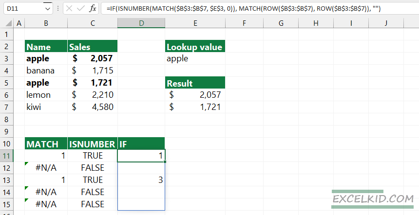
To generate the n-th smallest row number, use the SMALL function.
=SMALL(IF(ISNUMBER(MATCH($B$3:$B$8, $E$3, 0)), MATCH(ROW($B$3:$B$8), ROW($B$3:$B$8)), ""), ROWS($A$1:A1))The last part of the formula uses the ROWS function and returns the following result:
=SMALL({1;"";3;"";"";}, 1)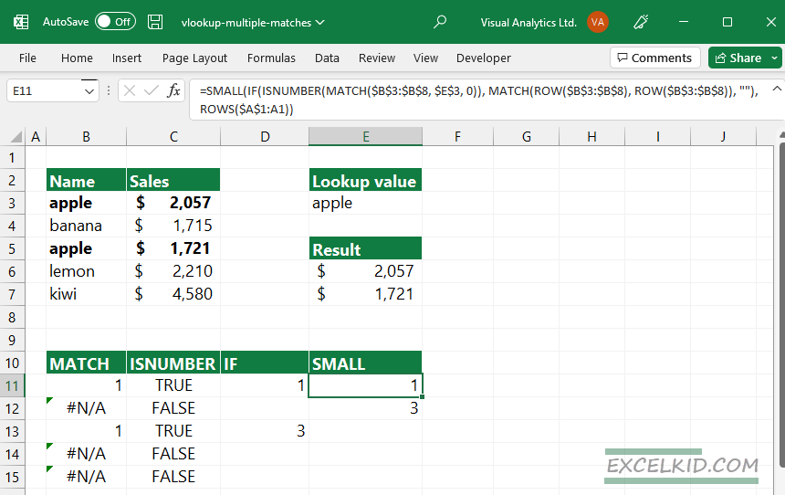
Finally, the INDEX function will return the matching records based on the row and column numbers:
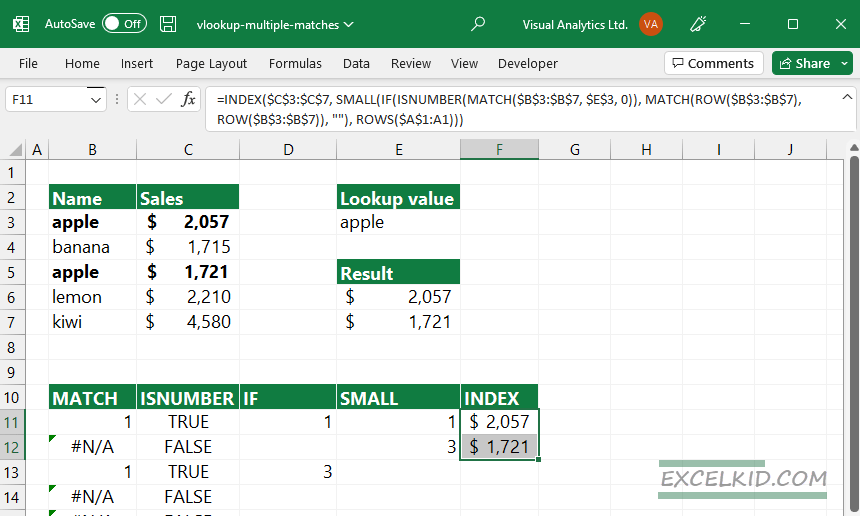
As a result of the formula, Excel displays all corresponding values if the lookup value is “apple”.