If you are working on an Excel dashboard, it is worth creating great-looking navigation. Everyone loves great UX! In today’s guide, I will show you how to build an interactive settings menu for your spreadsheet.
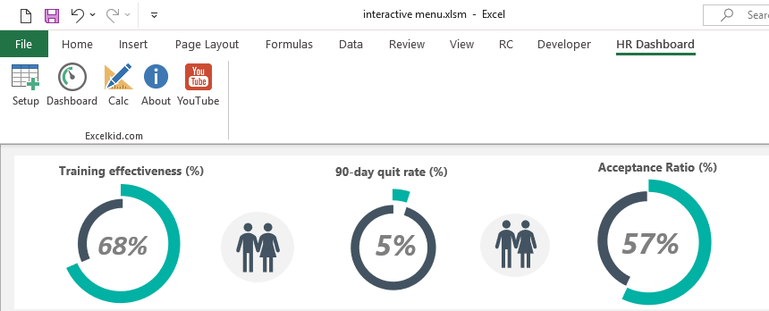
Take a close look at the picture below! Take a closer look at the picture below! This simple menu lets you interact with your Worksheets using clickable buttons and icons. It looks great.
Build an interactive settings menu
Step 1: Plan the menu structure
- Check how many worksheets you want to show
- Design the buttons for all Worksheet functions
In the example, I’ll show you how to quickly build an interactive setting menu to manage your Worksheets. OK, let us start the work! I’ll use three sheets based on the design rules: ‘Dashboard,’ ‘Data,’ and ‘Calculations.’
Step 2: Pick the icons for the interactive settings menu
I’ll choose the proper icons. We have three Worksheets, so we must select three icons to control the Workbook. I will prepare two additional icons because I want to add two extra functions (link to my About page and YouTube channel page).
It’s a great solution to control your spreadsheet from the ribbon.
Here are my icons:
Step 3: Download a custom UI editor
In this section, we will show you the steps to create an interactive settings menu:
- Close Excel and Open the Workbook for editing
- Add a CustomUI.xml part to your Workbook
- Add custom buttons and icons for the menu
- Check the syntax and validate the code
- Add callbacks (small macros)
Let’s see the details:
At first, we need a small app to edit the XML header. Download the latest version of Office Ribbon X Editor from Github. Then, move the archive to your Documents folder and extract the zip file content.
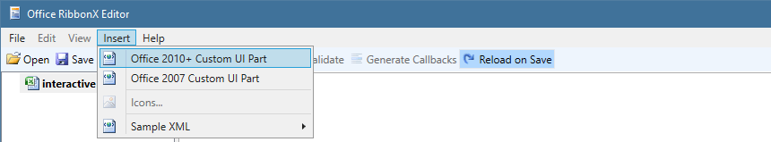
First, close Microsoft Excel, start the Editor, and open the Excel file that you want to edit:
Click on the Insert menu and choose the Office 2010+ Custom UI Part from the menu.
Step 4: Edit the XML header
Please copy the code and paste it into the CustomUI14.xml section.
Don’t worry; you can edit the menu if you download the example.
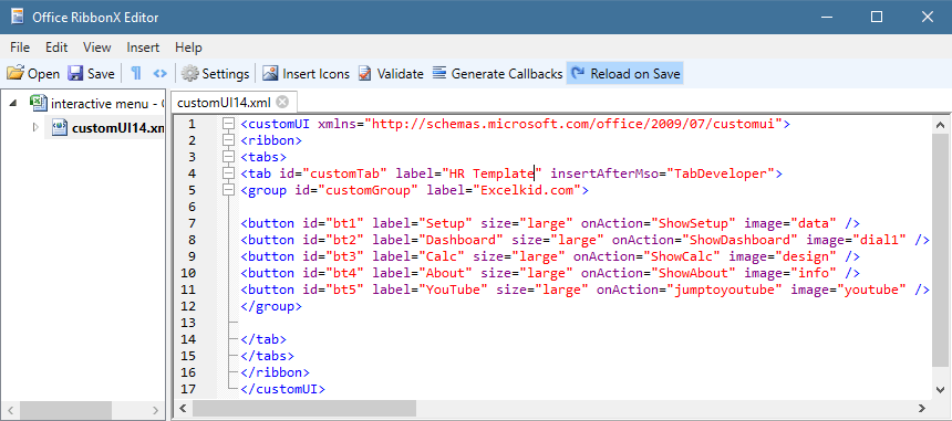
Just a few words about the variables:
- Tab: The new Tab will appear on the ribbon; in this case, the HR template
- Button ID: all buttons have a unique ID from btn1 to btn5
- label: you can define the labels freely
- onAction: call the macro from Excel
- image: the name of the inserted icon
Step 5: Insert icons
The next step is to insert your custom icons.
The best size is 32×32 pixels, and we recommend you use a transparent ‘PNG’ format.
Click on the Insert tab and choose icons. Next, locate the folder that contains your PNG files and click OK.
Step 6: Create callbacks for Worksheet selections
So, you want to manage your worksheets from the ribbon. To create a callback, open the Visual Basic Editor window by clicking Alt + F11.
Insert a new macro.
This snippet will activate the selected Worksheet.
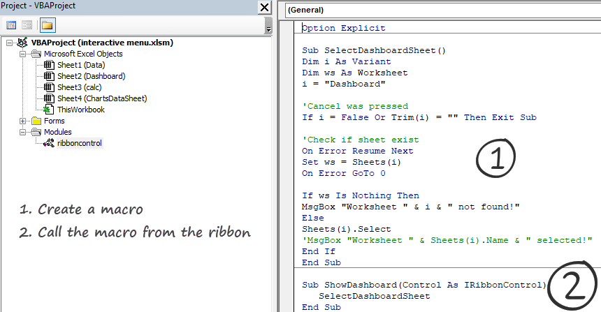
Finally, add a small Sub to call the macro from the ribbon. That’s all!
Important: Repeat these steps for all Worksheets and save the Workbook in xlsm or xlsb format.
Thanks for being with us today!
Additional resources: