Discover how to drill down into a Pivot table in Excel. Then, let us take a closer look and learn how to use the Quick Explore function.
Is there a tool to help us see behind the summed-up data? The answer is yes. Today’s article will introduce you to the drill-down feature capable of seeing under the hood.
Is it enough to display some corporate specifics (KPIs)? The answer is not as simple as we might think. If we make the report to a CEO, then the answer is yes. They can make the right decision based on a few key performance indicators. However, we must pay attention to every little detail.
How to Drill Down to show the Details
Pivot tables are your friends when working with Excel, especially when performing data analysis. First, let’s see how the structure of a table builds up. Every single value can contain one or more records.
Explanation: Let’s see an example of this. If we talk about a passport ID, one ID can belong to one person, called a 1:1 type connection. If we talk about the birth date, then the 1:N type connection is relevant. So we can easily see that more people can bear on the same day.
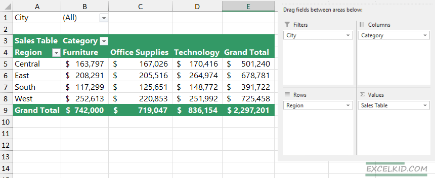
After this little sidetrack, let’s go back to the initial data set. In the figure below, we can see a sales table. At first glance, you know almost nothing about the value in cell C6 (East / Office Supplies). Therefore, use the drill-down feature to find out all the details!
How to extract Pivot table records?
We should use the drill-down method to create a dashboard in Excel. In the example below, we have summed up the data by regions and categories. Next, we want to display all the connecting records of cell C6.
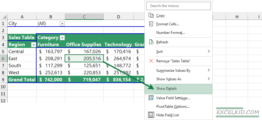
First, highlight one of the Pivot table cells containing data; after this, right-click the highlighted cell. Finally, choose the “Show Details” option from the appearing list.
Here is a tip to extract data quickly:
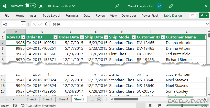
Instead of the Show Details command, there’s a lot faster solution to achieve the drill-down. First, highlight the cell value that we’d like to detail. Click on it twice, and the list is ready. Excel will automatically insert a new Worksheet that contains all “Office Supplies” records.
Workaround with Pivot table slicers
Be careful when you are using slicers. If we connect slicers, namely filters, to the Pivot table, we can be up for surprises. For example, using the drill-down function together with slicers can lead to false results in the versions of Excel before 2016.
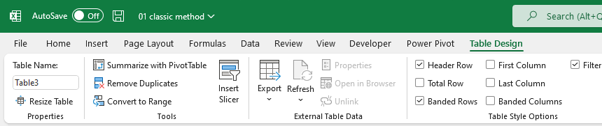
But they’re worth using in Excel’s newer versions, especially when we’d like to filter the table’s data even more before drill-down. To insert a new slicer, click on the Insert tab and choose the Slicer icon.
In the case below in the picture, the slicer contains all categories; if we would like to resolve the Grand Total in the E5 cell, all elements will be on the list.
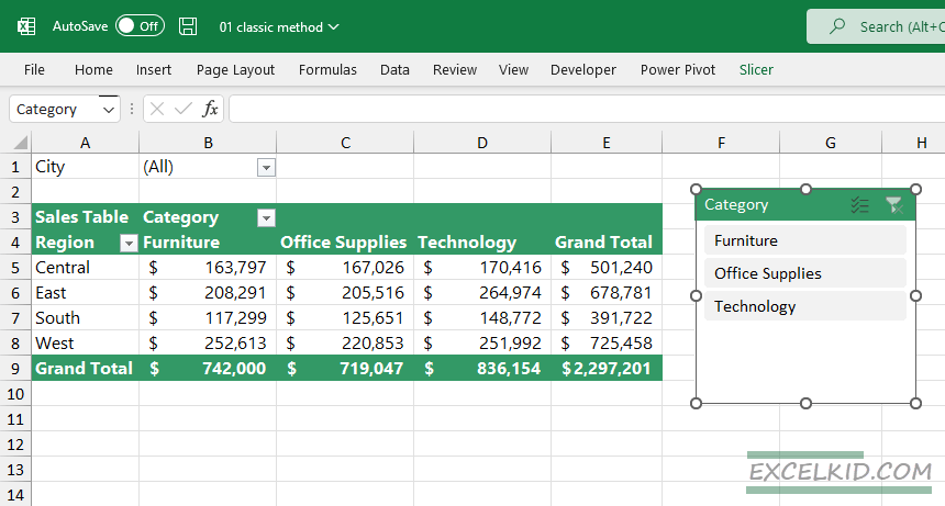
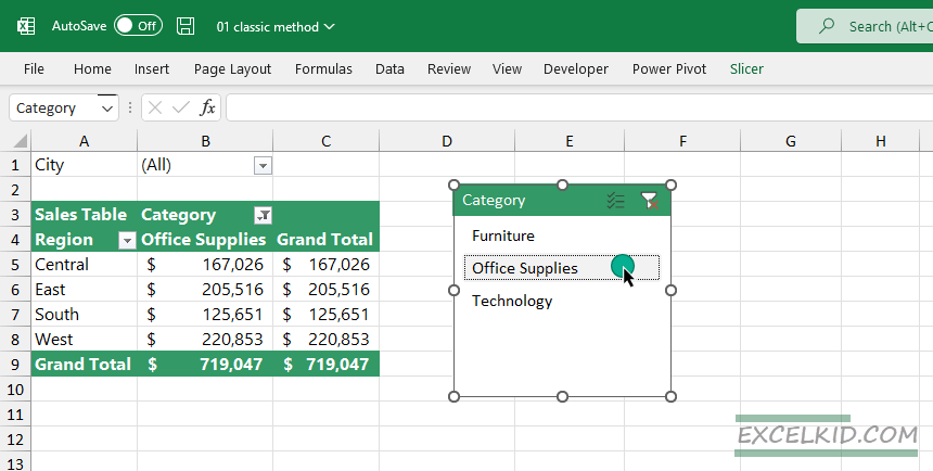
If you want to display a single category before the drill down, use the Pivot table slicer and click on the category name.
Keep an eye on the source data: There’s not much more frustrating when we have a missing connection between the source and the Pivot table. So what happens when the data of the Pivot table changes? Let’s see the nightmare of all analysts: data is not refreshing! And this can occur relatively quickly when we use an external data source. We cannot underline enough times that we only get a static list with the drill-down feature. The list is no longer connected with the original Pivot table!
Drill-down PowerPivot Data Model
This section will show you how to build a small data model using tables and PowerPivot. You’ll get an overview of the Quick Explore feature with a few clicks.
Build the data model
Quick Explore is a perfect solution in Excel if you want to drill down into the details. However, it’s good to know: you have to use Excel 2013 or above to apply this action.
In the example, we have sales-related data tables on the Tables worksheet.
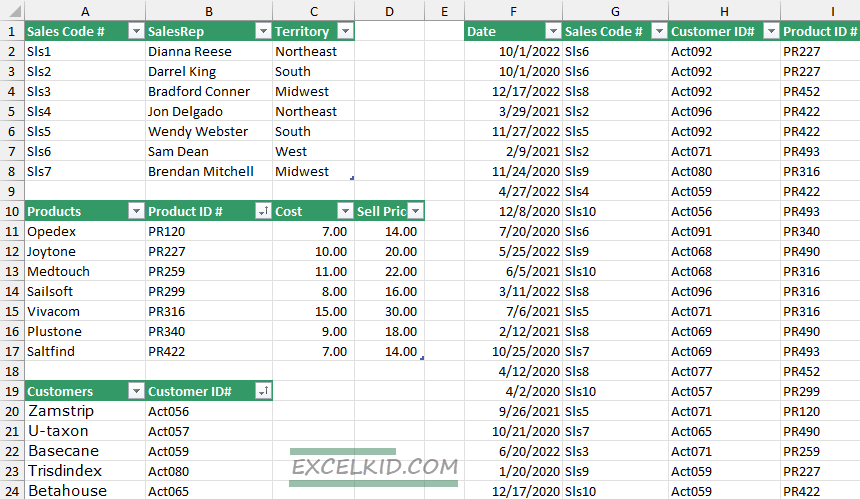
Let’s create relationships between tables first. Select the range and add the selected table from the Worksheet to the Data Model.
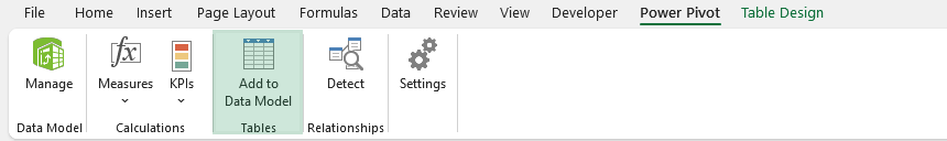
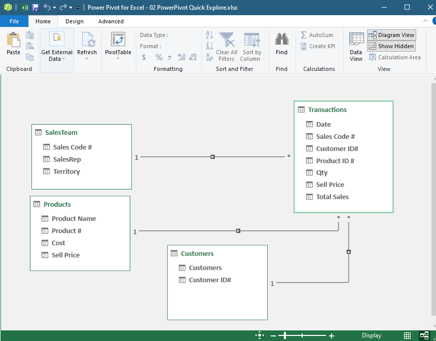
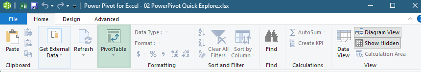
Now create a Pivot Table from the source tables. On the PowerPivot window, click the PivotTable icon. The structure will be summarized and grouped into a new Worksheet.
Drill down Using the Quick Explore Function
Finally, we will show you how to use the Quick Explore function. On the new Worksheet, click on a cell containing data; the Quick Explore icon appears.
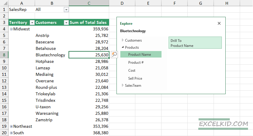
Select one field from the available options to drill down into the details. In this example, we want to extract the related product names of cell C8. The value is $25630 for the customers of BlueTechnology in the Midwest region. Choose this option from the Explore window.
Excel will rebuild the Pivot table and transform it. Check the top-left corner and the filters. The pivot table is now restructured and provides details about the selected cell. Use the Ctrl + Z keyboard shortcut to back your original table structure.
Additional resources: