
The scroll bar in Excel is one of the most useful tools in Form Controls. Using it will save time and get more space if you are using it. The most significant advantage comes when you work with a large data set. You can manage any size list in a small area using scroll bars.
Sounds good!
Do you still remember the rule of the one-page dashboard? In some cases, you need to show data in a small section of your Workbook. Get free spaces using the scroll bar, and it’s valuable. From now on, you can use great charts!
In today’s step-by-step tutorial, we’ll quickly show you how to manage a large dataset.
How to create a Scroll Bar in Excel
In the example, we will work with a large data set. The list contains 30 elements. Our task is to create a list that only includes ten elements and interactive mode.
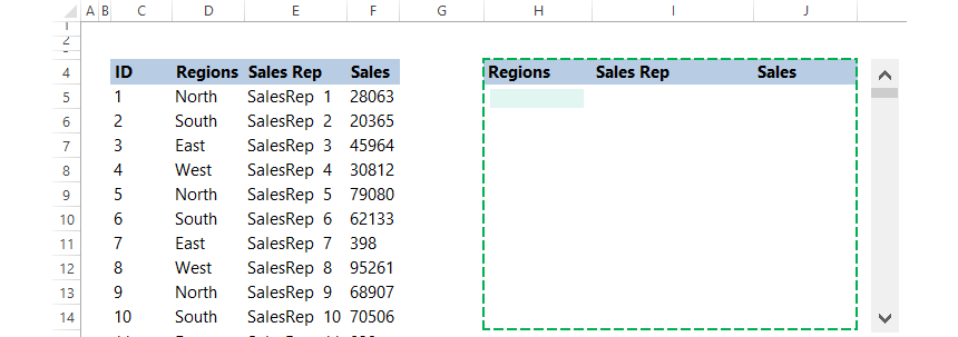
The trick is to show all values in this window using the scroll bar. The result will look like this:
Steps to create a dynamic list using Scroll Bar
Step 1: Prepare Data
First, let’s take a look at the data table. Create a list that contains 30 elements. The list is a simplified sales database.
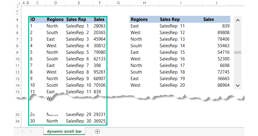
The table contains the following fields:
- Regions: the name of the place where the given manager works
- Manager: the name of the managers; we filled the columns with names
- Sales: the income that the given sales rep generated
Step 2: Locate the Developer Tab
Go to Developer Tab –> Insert –> Scroll Bar under the Form Control section
Tip: If you cannot find the Developer Tab, enable it.
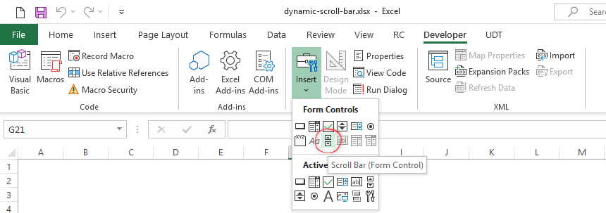
Step 3: Insert a Scroll Bar
Click on the Scroll Bar button. You can find it in the Form Controls section. To insert a Scroll Bar, click anywhere in the active Excel worksheet.

Step 4: Format the Scroll Bar
Right-click on the control. Click on ‘Format Control.‘ The Format Control dialogue box will appear.

In the Format Control dialogue box, go to the ‘Control’ tab and make the following changes:
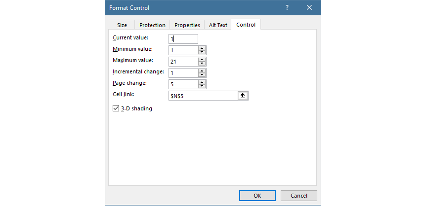
- Current Value = 1
- Minimum Value = 1
- Maximum Value = 21
Explanation: The maximum value is 21 because we will display ten elements in the list. You can get the idea that if the value of the N5 cell is 21, then the displayed values in the list will be between 21 and 30.
We want to show only ten rows, so the setup looks like this:
- Incremental Change = 1
- Page Change = 5
- Cell Link = $N$5
Explanation: Let’s talk about the N5 cell! We have linked this cell to the scroll bar. The value of the cell will vary between 1 and 21. Its role is vital because this will be one of the parameters of the OFFSET function. Next, we will fill out the now empty table.
Set the scroll bar’s size and place it on the right-hand side of the table. The picture below shows you what the table looks like after the action.
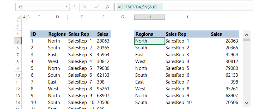
Next, write the following into the H5 cell:
=OFFSET(D4;$N$5;0)
As a result, we get the first element of the “Regions” column. Finally, copy this formula into all of the empty cells! And we are done with the dynamic list using the scroll bar and table. You can see this in the following picture:
What will make the list dynamic?
The OFFSET formula uses the D4 cell of the original list as a benchmark. Then, with the help of the N5 cell, it determines the appropriate position. But what is the correct position?
In the N5 cell (as we mentioned before), the values vary between 1 and 21. If we move the scroll bar up and down, then the value of the N5 cell will change.
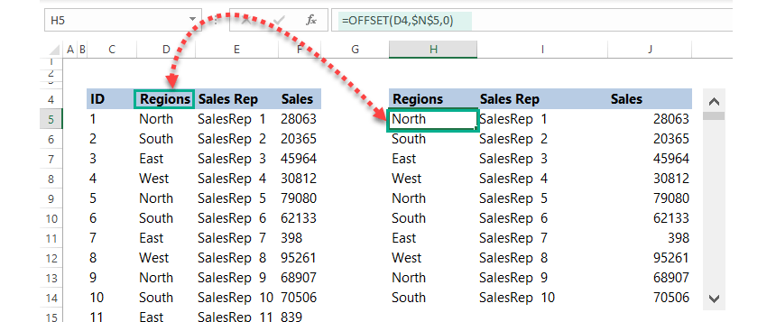
Evaluate the =OFFSET(D4;$N$5;0) formula!
We use the D4 cell as a base for a benchmark. Currently, the value of the N5 cell is 1. This value will go into the H5 cell, one cell away downward from the D4 cell.
Working with the OFFSET formula
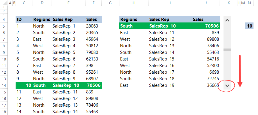
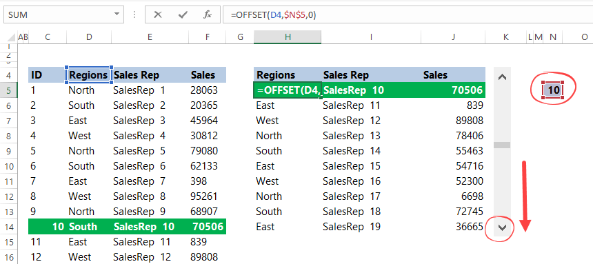
Now let us move the scroll bar so that the original list’s tenth element is the new list’s first item! It can be hard to imagine at first, so take a look at the picture below, and everything will be clear:
Let’s see what has changed!
The following formula gets the value of the H5 cell:
=OFFSET(D4;$N$5;0)
How can this be when the formula didn’t change? The formula did not change, indeed, but the value of the N5 cell did. Because of the downward movement of the scroll bar, its value has changed from 1 to 10. How did this affect the result?
Okay, take a closer look at the data set! The starting point is again the D4 cell. The value of it is 10. So, we jump exactly ten rows downward as the OFFSET formula’s effect starts from the D4 cell. Now, the new list’s first position will be the old list’s tenth element.
We show this in the following picture; most of us use a visual type:
Conclusion
The Form Controls group supports many useful tools in Excel. Stay with us in the future; soon, you can meet with new Excel tips and tricks! For example, you can try how the scroll bar works.