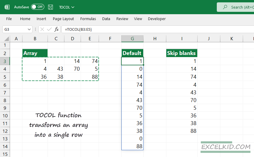
The TOCOL function flattens an array or range into a single column. By default, keep all values and scan left to right.
The function allows for the functionality we were missing from the FLATTEN function and works even more smoothly. Until now, there was no native FLATTEN function support in Microsoft Excel; it was available only in Google Sheets.
Syntax, Arguments
TOCOL function syntax:
=TOCOL(array, ignore, scan_by_column)
The function uses the following arguments:
- array: the array that you want to flatten to a single column
- ignore: options to manage blanks, errors
- scan_by_columns: scan direction; TRUE (column) by default, FALSE (row)
The “ignore” and “scan by columns” arguments are optional.
| Ignore mode | Usage |
|---|---|
| 0 (default) | Keep all values (0, blank, error) |
| 1 | Ignore blank cells in a range |
| 2 | Ignore formula errors |
| 3 | Ignore blank cells and errors |
The scan_by_column arguments control the read direction. By default (TRUE or 1), the TOCOL function reads the values from left to right by row. The function scans the data from left to right until the last column is reached in the first row. After that, TOCOL repeats the step above until the last value in the last column is reached.
If you want to change the read direction, set the argument value to 0 or FALSE. In this case, TOCOL will read values using the top-to-bottom order and keep the columns untouched.
How to use the TOCOL function
The purpose of using the TOCOL function is to create a new column. In a nutshell, you can merge multiple ranges into one array. For example, counting unique values in a range in Microsoft Excel is useful, even if we are working with non-contiguous ranges.
Let us see a few examples!
TOCOL function: Basic usage without optional arguments
In the picture below, we use the function without the optional arguments. The TOCOL function transforms the B3:D5 range into a single column and reads the data from left to right.
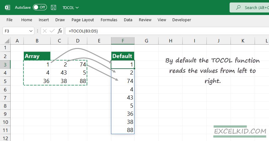
The formula in cell F3:
=TOCOL(B3:D5)The function transforms the 3×3 array into a 9×1 array.
If you want to convert the range into a 1×9 row, use the TRANSPOSE function.
Skip blanks and errors in an array
The source range contains formula errors and blank cells in the following example. You can easily control the output column using the TOCOL function’s second argument.
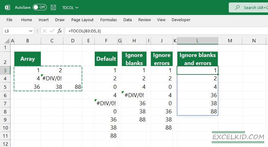
We show all possible settings for the ignore argument in the picture above:
Formulas:
=TOCOL(B3:D5) --- // default usage
=TOCOL(B3:D5,1) - // ignore blanks
=TOCOL(B3:D5,2) - // ignore errors
=TOCOL(B3:D5,3) - // ignore blank cells and formula errors
Working with non-contiguous ranges
My personal favorite feature is that the TOCOL function works smoothly with non-contiguous ranges!
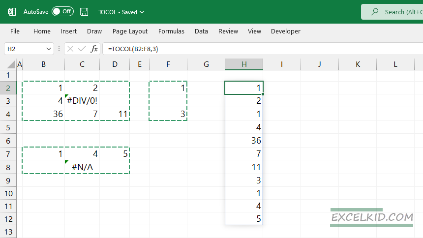
In the example, we want to merge three separate ranges into a single column.
The formula in cell H2:
=TOCOL(B2:F8,3)Using 3 as a second argument, the TOCOL function will create a clean, easy-to-understand output.
Scan by columns argument
The TOCOL function fills the new column by reading values from left to right. If you want to keep the structure of the original columns, set the scan_by_column argument to TRUE (or 1).
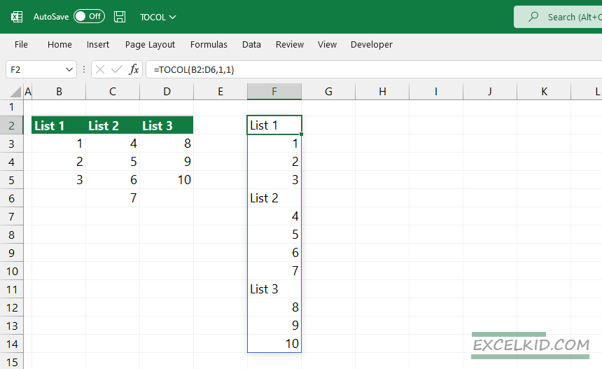
The formula in cell F2:
=TOCOL(B2:D6,1,1)