How to SUM top N values in Excel

Learn how to sum the largest n numbers in a range – sum top n values in Excel – using the SUMHIGH function.

Instead of using complex formulas based on LARGE and SUMPRODUCT functions, it is time to learn how to use the SUMHIGH function. With its help, you can build easy-to-read formulas without struggling.

SUM Top N values in a range

Steps to sum the top N largest numbers in Excel:

Use the SUMHIGH(range, n) function
Select the range that contains numeric values
Enter a number as a second argument to summarize the top N largest numbers in a range.
The formula will return the sum of the top N largest value

Generic formula: How to use the SUMHIGH function

Excel does not contain the SUMHIGH function by default. Instead, install our function library, DataFX, which contains various user-defined functions. SUMHIGH has a simple syntax, and it uses two required arguments.

Syntax:

=SUMHIGH(range, n)

Arguments:

Range: the range that contains numeric values
N: an integer type variable for the top N calculation

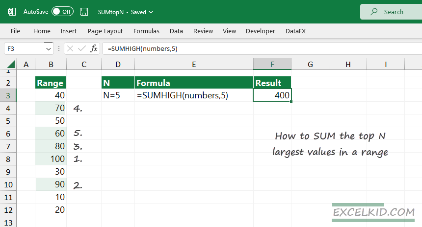
In the example, you want to find the top 3 largest values in the range B3:10, then summarize them. Create a named range! Select range B3:B10, then use the name box to add a name to a range, in this case, “numbers”.

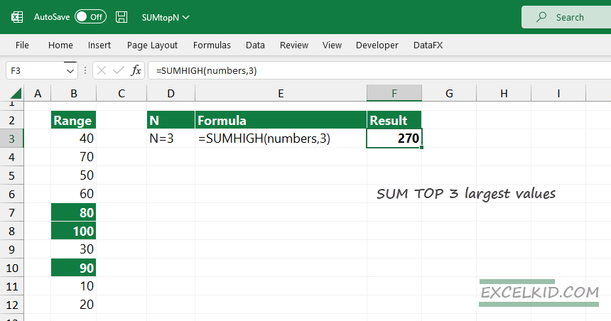
Enter the formula in cell F3:

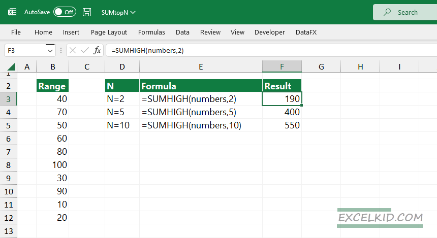
=SUMHIGH(numbers, 3)

Here are some examples to sum the top N largest value in a range:

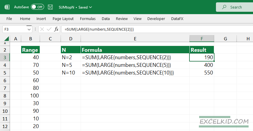
=SUMHIGH(B3:B9, 2)  // returns the sum of the top 2 largest number
=SUMHIGH(B3:B9, 5)  //returns the sum of the top 5 largest number
=SUMHIGH(B3:B9, 10) //returns the sum of the top 10 largest number

The next chapter section will show you another method for Excel users who are unfamiliar with user-defined functions.

Download the practice file.

Workaround with LARGE and SUMPRODUCT functions

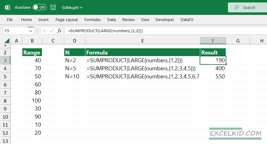
Without user-defined functions, you have to use the LARGE and SUMPRODUCT functions to summarize the top N largest numbers in a range.

Explanation:

By default, the LARGE function returns a single value. To create a return array, use the {1, 2, 3, 4, 5} constant when looking up the top 5 largest values.

Formula:

=SUMPRODUCT(LARGE(numbers,{1,2,3,4,5}))

As usual, evaluate the formula from the inside out:

=LARGE(numbers, {1, 2, 3, 4, 5}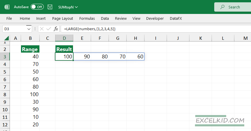

The result is a horizontal array that contains the top 5 largest values. The SUMPRODUCT function will use the result array as an argument:

=SUMPRODUCT(100, 90, 80, 70, 60) =400

SUM the largest N numbers using the SEQUENCE function

With Microsoft 365 (Excel 365), you can use the SEQUENCE function to generate an array using a single step and replace the SUMPRODUCT function with a simple SUM.

Formula:

=SUM(LARGE(numbers,SEQUENCE(n)))

To summarize the five largest values in a range, use the formula below:

=SUM(LARGE(numbers,SEQUENCE(5)))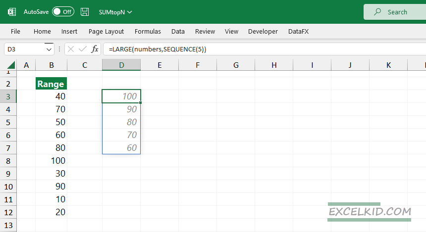

LARGE and SEQUENCE functions vertical array

The formula returns a vertical array containing the largest n values. In this case, n=5. To put the result into a single cell, use the SUM function.

Additional resources:

Functions