Sum last n columns

To sum last n columns in a range or a table, you can use the SUMCOLUMNS function in Excel instead of long formulas.

How to Sum last n columns in Excel

1. Write the formula in cell B3
2. =SUMCOLUMNS(B10:B20, n)
3. Press Enter
4. The function will return the last n columns in the range

SUMCOLUMNS function

SUMCOLUMNS is a user-defined function that lets you write a simple, easy-to-understand formula when you want to sum the last n columns or first n columns in a selected range.

Syntax:

=SUMCOLUMNS(range, n, [optional TRUE or FALSE])

Arguments:

The function uses two required and one optional argument.

• “Range”: range of cells that contain numeric values.
• “n”: the number of columns you want to sum.
• “firstColumns”: optional argument. In the case of TRUE, the function sums the last n columns. In the case of FALSE (default), the function will sum the last n columns.

Example to sum last n columns

In the example, we have 7 columns in the B3:H10 range, and the goal is to sum the last 3 columns.

Configure the arguments:

• Range = B3:H10
• n = 3
• firstColumns: We do not use the optional argument since the default value is FALSE.

Formula:

=SUMCOLUMNS(B3:H10,3)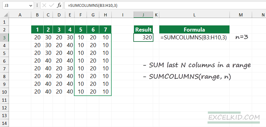

Workaround with SUM and FILTER Excel functions

What if you want to sum the last n columns in Excel and are unfamiliar with user-defined functions? The following method uses the SUM, FILTER, COLUMN, and COLUMNS functions.

Generic formula:

=SUM(FILTER(range, COLUMN(range)>COLUMNS(range)-(N+1)))

In the example, the range is B3:H10 and N=3; the formula looks like below:

=SUM(FILTER(B3:H10, COLUMN(B3:H10)>COLUMNS(B3:H10)-3+1))

Evaluate the formula from the inside out:

=COLUMN(B3:H10)>COLUMNS(B3:H10)-3+1 

The expression returns an array that contains boolean (TRUE and FALSE) values:

{FALSE, FALSE, FALSE, FALSE, TRUE, TRUE, TRUE}

This array will be the second argument of the filter function:

= FILTER(B3:H10, {FALSE, FALSE, FALSE, FALSE, TRUE, TRUE, TRUE}) 

The FILTER function returns a filtered range that contains the last N=3 columns:

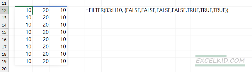
Finally, the SUM function calculates the sum of values in the last n columns.

=SUM(FILTER(B3:H10, COLUMN(B3:H10)>COLUMNS(B3:H10)-3+1))

The result is 320, which is equal to the SUMCOLUMNS function result.

How to sum first n columns

1. Write the formula in cell B3
2. =SUMCOLUMNS(B10:B20, n,TRUE)
3. Press Enter
4. The function will return the last n columns in the range

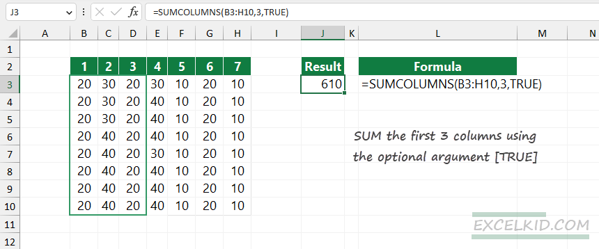
To sum the first n columns in a selected range, change the formula and apply the optional argument. Set the “firstColumns” argument to TRUE.

Formula:

=SUMCOLUMNS(B3:H10,3, TRUE)

Result:

If you want to use the SUMCOLUMNS function, copy and paste the code below into a new module.

Function SUMCOLUMNS(rng As Range, n As Long, Optional firstColumns As Long = 0) As Double
    Dim row, col As Long
    Dim sum As Double

    sum = 0
    For row = 1 To rng.Rows.count
        If firstColumns = 0 Then
            col = rng.Column + rng.Columns.count - n
            sum = sum + WorksheetFunction.sum(Range(Cells(rng.row + row - 1, col), _
            Cells(rng.row + row - 1, rng.Column + rng.Columns.count - 1)))
        Else
            col = rng.Column
            sum = sum + WorksheetFunction.sum(Range(Cells(rng.row + row - 1, col), _
            Cells(rng.row + row - 1, col + n - 1)))
        End If
    Next row

    SUMCOLUMNS = sum
End Function

Additional resources

• SUM every nth column