To count rows that contain specific values, apply the ROWCRT function or use a formula with the MMULT, TRANSPOSE, COLUMN, and SUM functions.
How to count rows that contain specific values?
- Type the formula =ROWCRT(B3:D12,40) in G3.
- Press Enter
- The formula will count the number of rows that contain the specified value.
ROWCRT function is a powerful UDF; look at our add-in section and download it to improve the built-in function library in Microsoft Excel. With its help, you can write short, descriptive formulas.
Example
In the example, the data set is in B3:D12. First, create a named range; select the range, jump to the name box, and add a descriptive name to a range, for example, “values”.
The goal is to check the range based on criteria (=40) and count rows that contain the given value.
Formula:
=ROWCRT(values,40)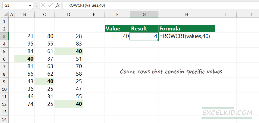
The ROWCRT function uses two arguments: “data” is the range of cells where we find the matching rows; “criteria” is a logical expression, “equal to x”.
The result is 4 since four rows contain the lookup value, which is 40.
Using the LAMBDA and BYROW functions
It is possible to calculate row numbers using the SUM, BYROW, and LAMBDA functions. For example, the following formula gets the number of rows in the “value” range that contains a specific value:
The formula in G3:
=SUM(BYROW(values,LAMBDA(row,--(SUM(--(row=F3))>0))))
Evaluate the formula from the inside out:
=LAMBDA(row,--(SUM(--(row=F3)))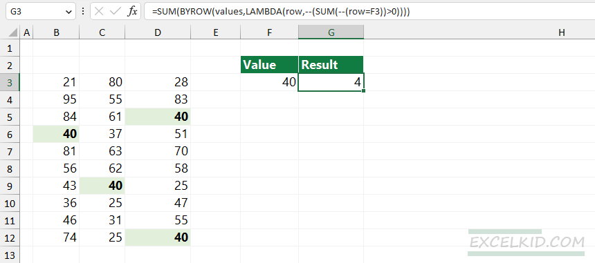
The LAMBDA function uses a horizontal array of values (row vectors) as input and checks the matching values based on the criteria (the value in cell F3). Next, the function uses the –(row=F3) expression and returns an array that contains boolean values. Using double-negative, you can convert boolean values to 0s and 1s. If the value is TRUE, we have a match in the given row.
=SUM(--(row=G4))>0.Finally, the BYROW function calculates the sum of values in a specific row; if the sum of the array is greater than 0, the formula returns 1, so we have a match in the given row.
Count rows that contain specific values using the MMULT function
It can happen that you do not want to use a quick, simple way to perform a complex task using user-defined functions. This section will show you a possible workaround with the MMULT function. The result will be a long formula, but we will evaluate it step by step.
Generic formula:
=SUM(--(MMULT(--(criteria),TRANSPOSE(COLUMN(data)))>0))Explanation:
- =COLUMN(data) returns an array that contains numeric values.
- =TRANSPOSE(COLUMN(data)) flips the column array into a row array.
- =–(criteria) returns an array of 1s and 0s, match=1.
- =–(MMULT(–(criteria)TRANSPOSE(COLUMN(data)))>0) formula multiplies the criteria array with the (transposed) column array. After that, it converts the result into an array that contains 0s and 1s. The conversion phase uses the double-negative method.
- =SUM(–(MMULT(–(criteria),TRANSPOSE(COLUMN(data)))>0)) formula sums the array that contain 0s and 1s.
The result is the number of rows that are met the given criteria.