Count cells that contain specific text

To count cells that contain specific text in Excel, you can use the COUNTTEXT, COUNTIF, or SUMPRODUCT functions.

How to count cells that contain specific text

1. Type the =COUNTTEXT(B3:B11,”X”) formula
2. Press Enter
3. The formula returns the number of cells that contain a specific text

COUNTTEXT is a powerful function; the goal is to count cells that contain one or more strings in the given cell. The main advantage of using the function is that you do not need to apply wildcards or create complex formulas.

Example

In the example, the data is in the range B3:B11. The range contains text values. For the sake of simplicity, create a named range; select the and add a descriptive name using the name box. From now on, “data” refers to B3:B11.

Here is the formula that counts the number of cells that contain a specific text, in this case, “x”).

=COUNTTEXT(data,"X")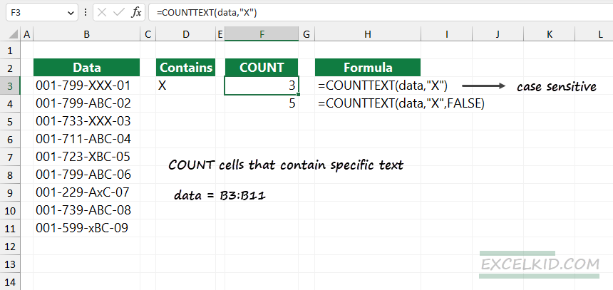

The function uses case-sensitive search by default, so the result is 3. In cell F4, we are using the third optional argument for non-case sensitive search (where the text contains “X” or “x” values. Therefore, set the third argument to FALSE.

Formula:

=COUNTTEXT(data,"X", FALSE)

In this case, the result is 5; COUNTTEXT counts the cells that contain “x” or “X”.

Note: The COUNTTEXT function is a part of our free Excel add-in, DataFX.

COUNTIF Function

If you are unfamiliar with user-defined functions, you can use regular Excel functions to count cells that contain specific text. However, this workaround needs attention; we will use a wildcard to create a formula.

Generic formula to count cells that contain a specific substring:

=COUNTIF(range,"*text*")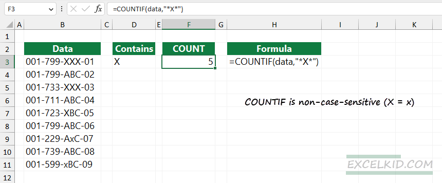

In the example, use the formula in cell F3:

=COUNTIF(data,"*X*")

The result is 5. The main problem with COUNTIF is that you can not control the case-sensitive search; the function always uses a non-case-sensitive search.

Count cells that contain specific text using SUMPRODUCT

In this example, we will show you a workaround with the SUMPRODUCT function using the boolean logic. The solution will provide case sensitive search (finally!).

Formula:

=SUMPRODUCT(--ISNUMBER(FIND("X",data)))

Evaluate the formula from the inside out. The FIND function is case-sensitive so that the function will identify “X” and “x” as different values. The formula uses a logical test.

=FIND(“X”,data)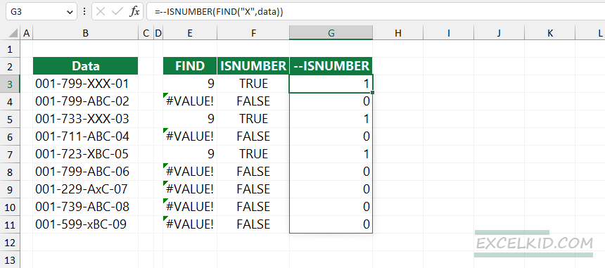

Use the FIND function because it gets the position of text in a text string as a number. In the example, the function returns 9 since the “X” character is in the 9th position of the given text.

=FIND(“x”,”001-799-XXX-01” = 9

If the “X” character is not found in the text, the function returns a #VALUE error. Next, the ISNUMBER function will check whether the cell contains a numeric value.

=ISNUMBER(FIND(“x”,data)

This formula returns an array that contains TRUE and FALSE, in other words, boolean values. To convert boolean values to 0s and 1s, use the double-negative method.

=--(ISNUMBER(FIND(“x”,data))
= {1, 0, 1, 0, 1, 0, 0, 0, 0}

Finally, the SUMPRODUCT function sums the matching values in the array, and the result is 3.

SUMPRODUCT({1, 0, 1, 0, 1, 0, 0, 0, 0}) = 3.

For a non-case-sensitive count, use the FIND function in the following formula:

=SUMPRODUCT(--ISNUMBER(SEARCH("X",data)))

Related Formulas

• Count cells that contain text
• Count cells not between two numbers
• Count if cells less than a given number