To SUM visible rows in a filtered list in Excel, use the SUMVISIBLE function or the built-in SUBTOTAL or AGGREGATE functions.
How to sum visible rows in a filtered list?
- Write the formula in cell B2
- SUMVISIBLE(A10:B10)
- Press Enter
- The function will return rows that are filtered out
The SUMVISIBLE function returns the sum of visible cells in a filtered list, even if some rows are manually hidden. In the next section, you will learn how the formula works.
Generic formula
=SUMVISIBLE(range)Example
In the example, we have a filtered list. Furthermore, we hide some rows manually to demonstrate how the function works.
The SUMVISIBLE function returns the SUM of the visible rows only. The main advantage of the function is that it uses a single argument.
We created a custom data set containing a manually hidden row (6) and rows filtered out using the header filter (rows 10 and 12).
Formula:
=SUMVISIBLE(D3:D12)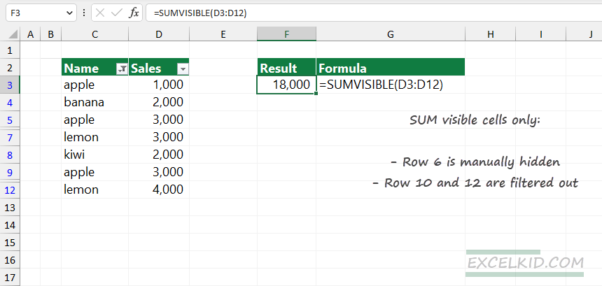
Note: the function is more user-friendly than other Excel functions; select the filtered range, and you will get the result quickly.
SUM visible rows using the SUBTOTAL function
The SUBTOTAL function uses two arguments to perform various actions (SUM, COUNT, AVERAGE, MAX, MIN).
Generic formula:
=SUBTOTAL(function_num, reference1, [reference2]…)SUBTOTAL can be useful to sum values in visible rows and ignore values hidden in the selected list.
Ignore filtered rows
Add “9” as a first argument to sum visible rows and ignore hidden rows:
=SUBTOTAL(9,D3:D12)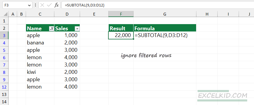
Explanation:
In the example, add “9” to the first argument (function_num); this number equals the SUM function in Excel. Then, use the D3:D12 range for the second argument (reference). Finally, apply a filter using the header to hide the values in rows 10 and 11.
The SUBTOTAL function will ignore the filtered rows in a range and returns with 22000; in other words, sum the visible rows only.
Ignore manually hidden rows
In the example, we hide rows 10 and 11 manually. In this case, use “109” as function_num. Next, select the D3:D12 range as a reference.
Formula:
=SUBTOTAL(109, D3:D12)The SUBTOTAL function will ignore the manually hidden rows in a range and return with 22000; in other words, it will only sum the values in visible rows.
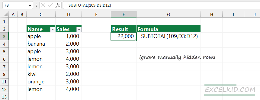
Note: if you want to sum visible rows in a range that contains manually hidden rows, do not use “9”. Always use “109” to get the proper result.
SUM visible rows with the AGGREGATE function
Let us see another method using the built-in AGGREGATE function and apply it to a filtered range.
Formula:
=SUBTOTAL(9, 5, D3:D12)Good to know the difference between the AGGREGATE and SUBTOTAL functions. By default, SUBTOTAL ignores values in rows hidden by a filter, and you need to use the “109” function number to ignore manually hidden rows.
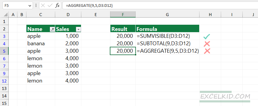
AGGREGATE uses three required arguments and ignores the rows that are manually hidden. Furthermore, you must use an additional argument to specify the criteria.