Subtraction formula in Excel

The tutorial shows how to use the subtraction formula in Excel. Learn how to subtract numbers, percentages, dates, and times easily.

This article is a part of our must-have guide on Excel Formulas.

Subtraction is a simple arithmetic operation. We all know that you will use the minus sign to subtract one number from another. Okay, how it works if you are using Microsoft Excel? What kind type of data can you subtract? Almost all: you can use numbers and percentages. Furthermore, subtraction is available for other data types like days, months, hours, minutes, and seconds. Believe it or not, you can use subtraction for texts too.

Let’s start and learn how to do it for almost all data types.

Table of contents:

• Excel Subtraction Formula
• How to Subtract cells in Excel
• Subtract multiple cells from one cell
• Subtraction formula for columns
• How to Subtract the same number from a column of numbers
• Subtraction formula for percentage
• How to subtract date and time in Excel
• Matrix subtraction formula (using arrays)
• How to subtract one text cell from another in Excel

Subtraction formula in Excel (apply minus sign)

In Excel, all formula starts with a ‘=’ (equal) sign. So, for example, to subtract two or more numbers, you need to apply the ‘-‘ sign (minus) operator between these values. That’s all, looks easy.

=number1 – number2

In the example, you want to subtract 33 from 50, use the simple formula and get 30 as the result of the equation:

=50 – 20

Steps to create the subtraction formula in Excel:

1. Select the cell where you want to get the result and type an equal sign (=)
2. Enter the first number
3. Type the minus sign
4. Add the second number
5. Press Enter to evaluate the formula

Tip: you can do multiple subtractions within one basic formula.

In the example, you want to subtract more than one number from 50. To do that, separate the numbers using a minus sign.

=50 – 20 – 10 – 5

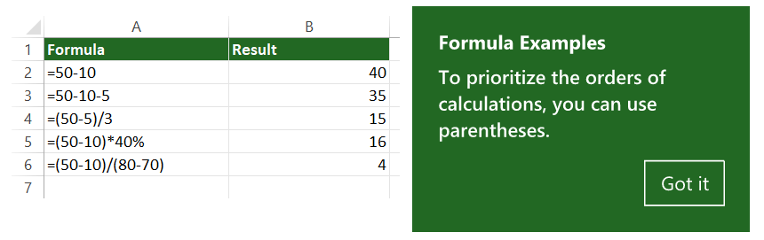
To prioritize the orders of calculations, you can use parentheses, like the example below:

=(50 – 10) / (10 – 5)

Let’s see a few formula examples:

How to Subtract cells in Excel

To execute a formula that subtracts one cell from another, use cell references:

=cell1 – cell2

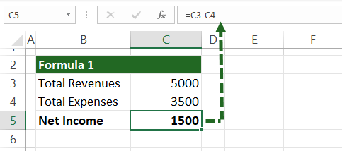
The following example shows how to subtract the number in cell C4 from the number in C3.

=C3 – C4

Forget to enter the cell references manually!

Instead, here are the steps to use subtraction between cells:

1. Select the output cell
2. Type an equals sign (=)
3. Click on the cell that contains the minuend (C3)
4. Type a minus sign (-)
5. Click on the cell that contains the subtractor (C4)
6. Press Enter to calculate the difference

Subtract multiple cells from one cell

There are three methods:

• use the SUM function
• apply the minus sign
• sum negative numbers.

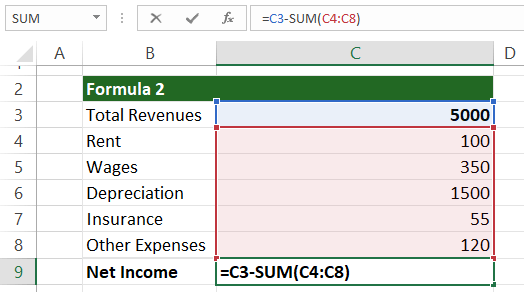
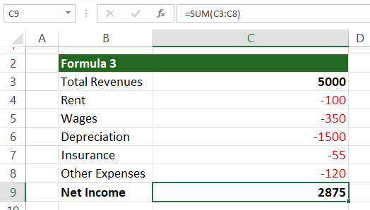
Example 1: Using the SUM function

The easiest way to subtract multiple cells from one is using the SUM function. First, add the subtrahends (C4:C8), then subtract from the minuend, in the example, cell C3.

=C3 – SUM(C4:C8)

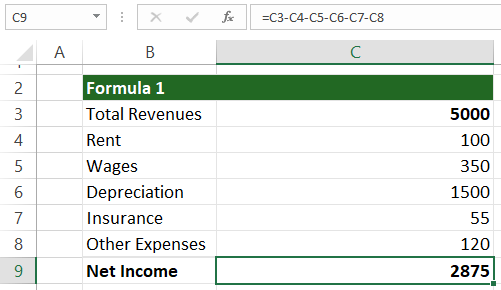
Example 2: Using the Minus sign

If you don’t want to use formulas, use the minus sign to subtract multiple numbers. In the example, you subtract cells C4:C8 from C3:

=C3 – C4 – C5 – C6 – C7 – C8

Example 3. The subtraction formula summarizes negative numbers

If you subtract a negative number from a positive number, the result will be the same as adding it. Use the SUM function to sum the positive and negative numbers.

=SUM(C3:C8)

Subtraction Formula for columns

The following example will show how to write a formula to subtract columns.

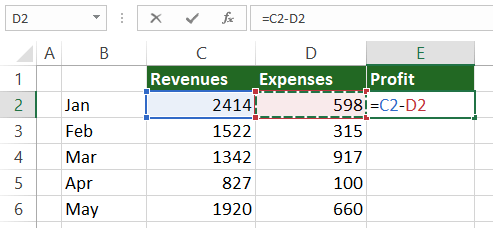
To subtract numbers from column D from the numbers in column C, enter the formula. But first, create a new column for the result in cell E2.

Type the formula for cell E2.

=C2-D2

After that, select cell E2 and copy the formula down using the cross sign.

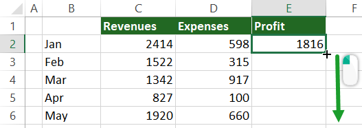
In this case, we are talking about relative references.

How to Subtract the same number from a column of numbers

In this example, you will use a fixed cell value, B9, as a subtrahend.

Steps to create a subtraction formula for cell D2:

1. Select cell D2
2. Type an equal sign
3. Select cell C2
4. Add a minus (-) sign
5. Select cell B9
6. Press F4

=C2 – $B$9

What’s the point? If you lock the cell using the dollar sign ($), you can create an absolute cell reference in Excel. From now on, the second part of the subtraction formula will fix.

Copy the formula down, and the result is correct in each row.

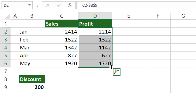
As a result of using absolute reference, the formula in cell D3 will change to =C3-$B$9, and so on.

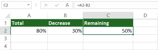
Subtraction formula for percentages

The subtraction between percentages is not rocket science, and the above-mentioned subtraction formula works fine. In the case of fixed values, use the classic method:

= 80% – 30%

You can use cell references, too by using the following formula:

= A2 – B2

How to decrease a number by a percentage

In the example, you want to subtract a percentage from a number.

The formula looks like this:

=Number * (1- %)

For example, let us see how you can reduce the number in B3 by 25%.

Use the formula:

= B3 * (1-$C$3)

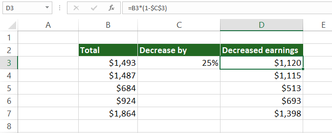
Because we are using absolute reference, it’s easy to copy the subtraction formula down.

How to subtract date and time in Excel

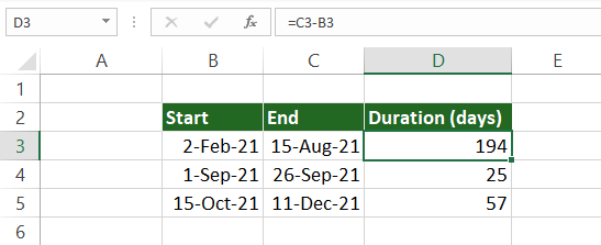
Subtraction formula for dates

Working with dates, it’s easy if you want to subtract one cell from the other. In the example, we would like to get dates in column D. The start and end dates are in cells B3 and C3.

To get the differences between two cells that contain date formats, use the minus sign in the subtraction formula:

= end_date – start_date

= C3 – B3

You’ll get the result in days.

Tip: It’s possible to subtract dates using built-in Excel functions. Use the DATE function to calculate the differences between dates!

The subtraction formula:

=DATE(2021,9,15) – DATE(2021,9,11) = 4

How to subtract time in Excel

You can create a time subtraction formula in Excel based on the date formula:

The syntax:

= end_time – start_time

= C3 – B3

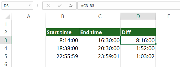
Now you have the result in D3. Copy the formula down to fill the column.

Matrix subtraction formula in Excel (using arrays)

Suppose that you have two matrices (with equal size), and you want to subtract the corresponding elements of the range.

For the sake of simplicity, here is an example:

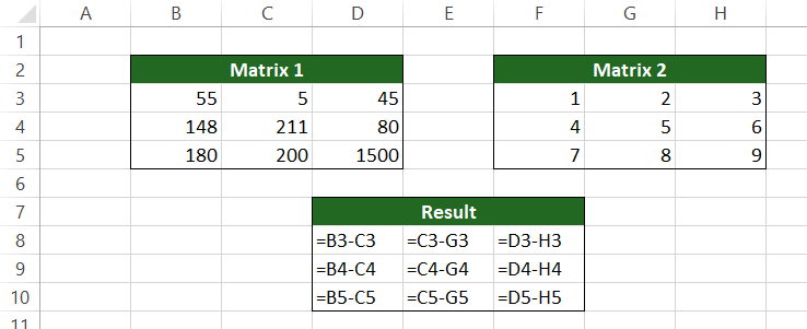
This method is a bit slow, so we are looking for a faster and better solution.

Steps to subtract matrix2 from matrix1 using an array formula!

1. Select cell D8
2. Enter the formula = (B3-D5) – (F3:H5)
3. Use the Ctrl + Shift + Enter to create an array formula

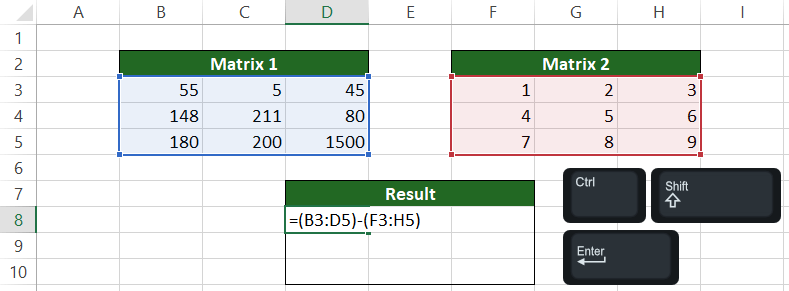
Let us see the results of the subtraction In cell D8! Check the formula bar! The subtraction formula is surrounded by {curly brackets}.

Copy the formula to fill the remaining cells.

How to subtract one text cell from another in Excel?

If you are familiar with VBA, we have some good news. Use the TEXTSUBTRACT function to subtract characters in one string from another string:

Function textSubtract(startString As String, subtractString As String) As String


Dim charCounter As Integer
For charCounter = 1 To Len(subtractString)

  startString = Replace(startString, Mid(subtractString, charCounter, 1), "")

      Next charCounter

  textSubtract = startString

End Function

How to add a new code? First, open a new Workbook, and press Alt + F11 to open the VBE window. Then, insert a new module and add the code as mentioned above. Finally, save the Workbook in .xlsm format.

Tip: if you have found the ‘Excel found a problem with formula references in this Worksheet,’ try to fix it using absolute references.