Using a Panel chart (small multiples) is a great decision if you want to compare products or sales and show the data on the same scale. If you create dashboards in Excel, it is important to use space-saving methods and focus on the data.
Our step-by-step tutorial shows you how to create a panel chart from the ground up. Our goal is to compare the performance of two products using four locations.
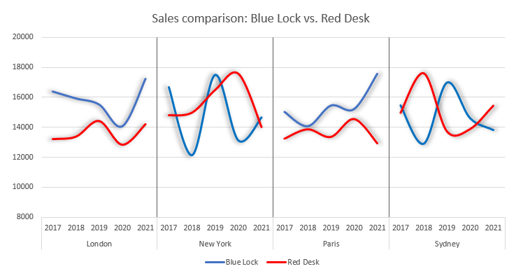
Here is a great template that uses a panel chart:
One more important thing: Excel does not support the panel chart in default. We need to follow custom steps to build it. If you are in a hurry, use our chart add-in. With its help, you can create the chart in seconds.
Steps to create a Panel Chart in Excel
Step 1: Arrange your Data
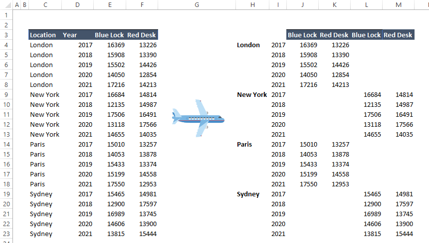
Before we take a deep dive into the details, let us see our data:
In the example, we will compare the data sets of the two software, ‘Blue Lock’ and ‘Red Desk,’ using four different regions in five years. Create the following structure for the panel chart.
We will apply pivot tables to manage data.
It is worth using Pivot Tables for consolidation or data extraction! You can create the output manually, but it can take a while.
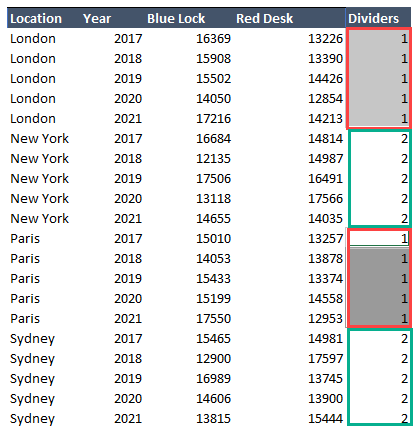
Step 2: Add a helper column to the table
The first trick is to add a helper column. It will play an important role if you are working with a Pivot Table. Add a new column in column G and enter ‘1’ for the range G4:G8 and G14:G18. Now use ‘2’ for range G9:G13 and G19:G23.
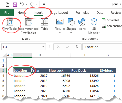
Step 3: Build a Pivot Table from the data
Steps to build a new Pivot Table:
- Select the range of cells, in this case, cell C3
- Click on the Insert Tab
- Click PivotTable.
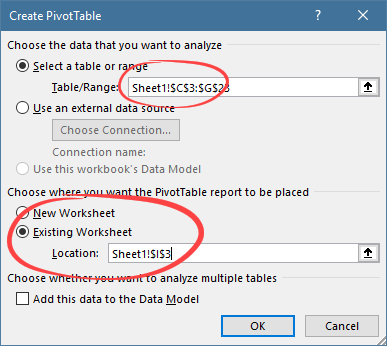
Now in the ‘Create PivotTable’ dialog box, apply the following settings. We want to manage the original data set and the new Pivot data in the same Worksheet. Use the ‘Existing Worksheet’ as a location. Click OK to close the window. In the example, place the new table to cell I2.
Step 4: Build a pivot table output using Fields
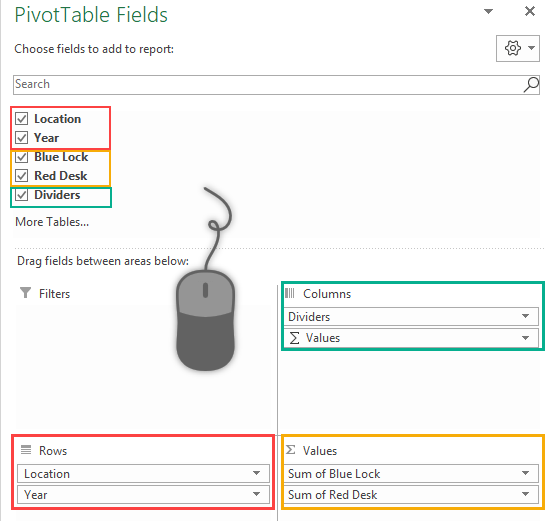
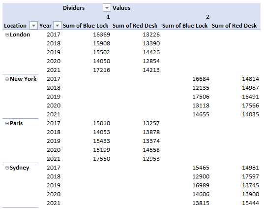
We have an empty Pivot Table. It is time to add data to the table. Click inside the Pivot Table, and add fields using the PivotTable Fields task pane. We need this structure to create the panel chart.
- Move the ‘Location’ and ‘Year’ to Rows.
- Drag ‘Dividers’ and drop to ‘Columns.’
- Add the ‘Blue Lock’ and ‘Red Desk’ to the ‘Values.’
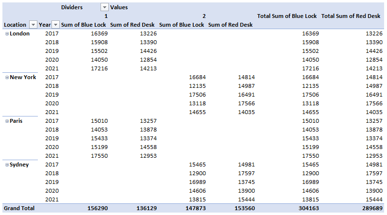
The table looks like this:
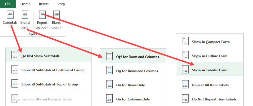
The table contains redundant records, so we need to remove subtotals and transform the data. Select a cell in the Pivot Table range and select The Design Tab.
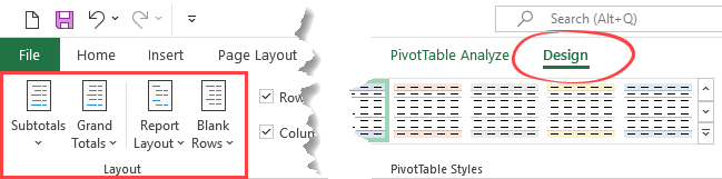
- Choose the Subtotals icon and remove subtotals using the ‘Do not show Subtotals.’
- Click on the ‘Grand Totals,’ select ‘Off for Rows and Columns.’ To hide Grand Totals
- Enable a custom view. Click on the Report Layout menu. Select ‘Show in Tabular Form.’
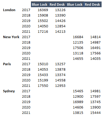
Our data looks much better!
Step 5: Extract data and add a Header
Copy the Pivot Table into a new location using the Paste Special command and add a new row that contains the header.
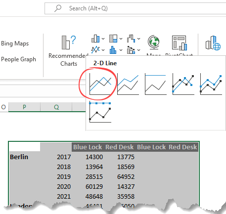
Step 6: Create line charts
To create a panel chart, we need to insert and combine line charts. Select the data and click on the Insert Tab. Insert a line chart by clicking the icon.
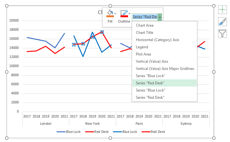
Step 7: Change the data series colors
The line chart contains different colors for each series. Apply a consistent color scheme. We will use the same colors for the same series.
Right-click on the chart and select ‘Outline.’ In this example, we will use blue for the ‘Blue Lock’ and red for the ‘Red Desk.’ If you use the context menu and the drop-down list, it is easy to select the series.
Step 8: Calculate the separator line positions
To improve the panel chart, we have to divide the line chart section into four parts. We will apply vertical error bars as separators. To plot the dividers, we’ll create a small table for additional calculations.
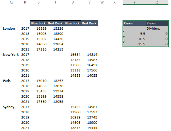
In the example, we will use the range Y4:Z8
- Leave the cell Y5 blank, and fill the cells using zeros in column Z.
- Enter the following formula in cell Y6. =COUNTA(R5:R9)+0.5
- Apply the =Y6+COUNTA(R10:R14) formula in cell Y7.
- For the cell Y8, use the =+Y7+COUNTA(R11:R15) formula.
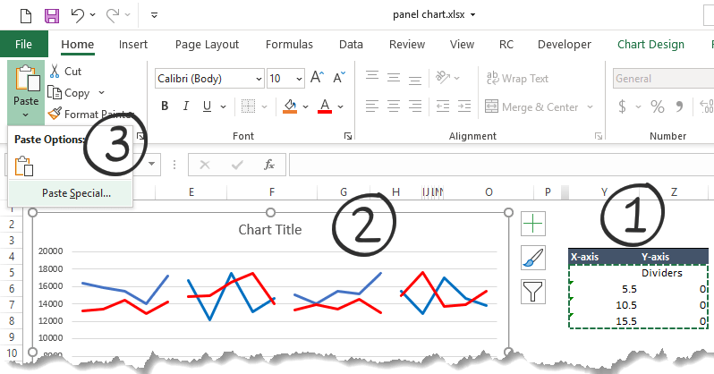
Step 9: Create temp series for Panel Chart
Follow the steps below to build a dummy series:
- Select and copy range Y5:Z8
- Click on the chart area.
- Go to the Home tab and select ‘Paste.’
- Use the ‘Paste Special’ command
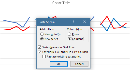
The ‘Paste Special’ dialog box will appear.
Make sure that the following checkboxes are checked:
- New series
- Columns
- Series Names in First Row
- Categories (X Labels) in First Column
Click OK to close the dialog box.
Step 10: Use Scatter Plots with straight lines
You can find the new series at the bottom-left corner.
Right-click and apply the ‘Change Series Chart Type’ command.
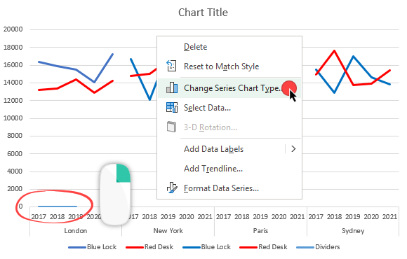
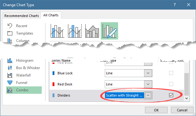
Select the Dividers series and apply a new chart type: ‘Scatter with Straight Lines.’
Step 11: Remove the unnecessary chart elements
It can take only seconds to clean up the chart.
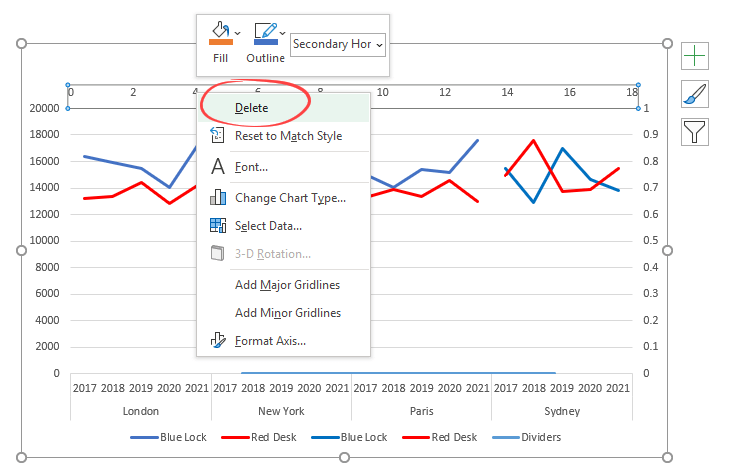
First, Right-click on the secondary axis, then click ‘Delete.’
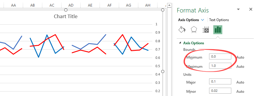
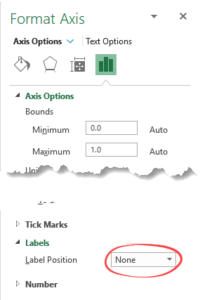
Right-click on the vertical axis!
Check the ‘Format Axis’ (Axis Options Tab) setup on the Task pane:
- Add ‘0’ for Minimum Bounds
- Add ‘1’ for Maximum Bounds
To hide the axis scale, jump to the Labels section. Then, change ‘Label Position’ to ‘None.’
Step 12: Use error bars as Panel Chart separator
The panel chart looks much better! Let us see how to add error bars.
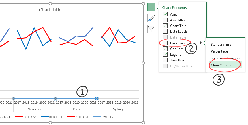
- Select the series ‘Dividers’ at the bottom of the chart area
- Under the Chart Elements menu, click the plus sign
- Hover the mouse over the ‘Error Bars,’ then click ‘More Options.’
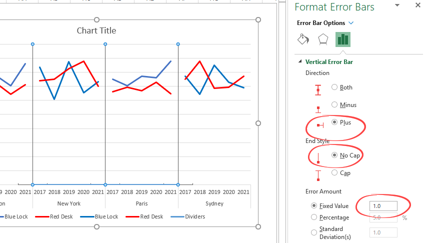
Change the vertical error bar settings in the Format Error Bars task pane to modify the dividers:
- Select ‘Plus’ for direction.
- Apply ‘No Cap’ for End Style
- Add ‘1’ as a ‘Fixed Value’ under Error Amount Group
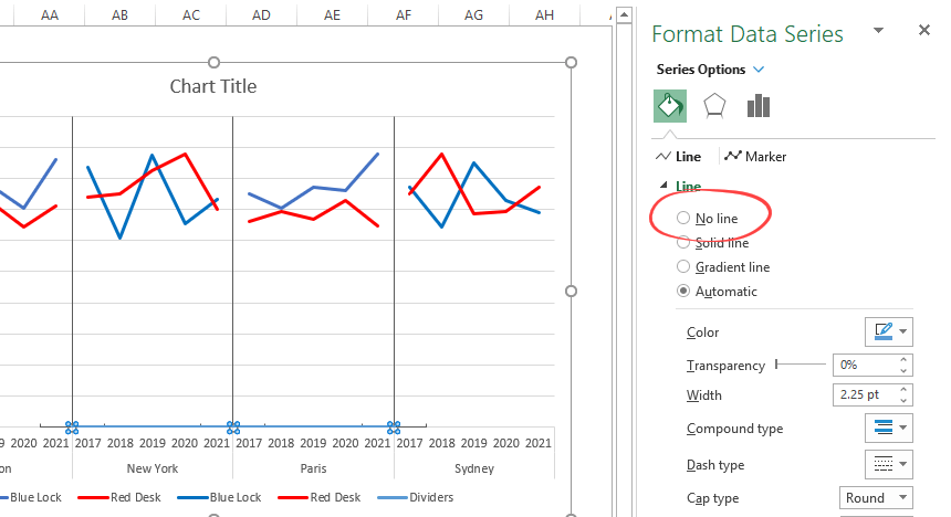
Step 13: Clean up the Chart (Part II.)
The last step is to clean up the chart. Select the ‘Dividers’ series and click on ‘No Line.’ You can hide the horizontal error bars, too, using this method.
To improve your panel chart, enter a title and remove the duplicated product names from the legend. Then, add a shadow for the lines and/or use smoothed lines.
Here is the panel chart!
If you want to learn more about chart templates, visit our guide.