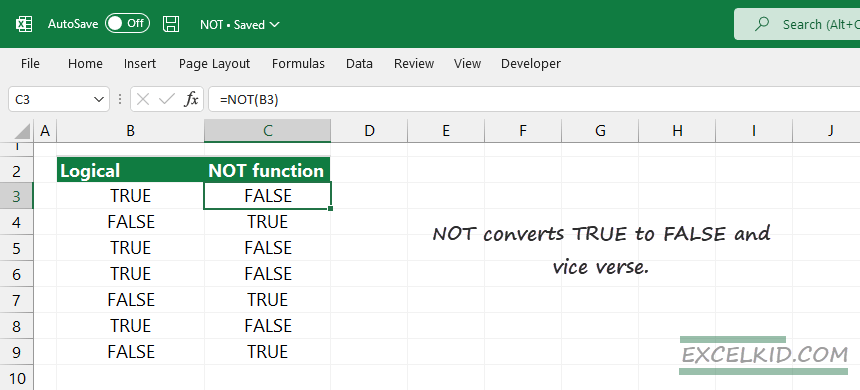
The Excel NOT function returns a reversed boolean value of a given logical or boolean value. NOT converts TRUE to FALSE and vice versa.
Syntax and arguments, return value
The syntax is simple:
=NOT(logical)Argument: The function uses one argument: “Logical”, the value that the function will convert to TRUE or FALSE. Ensure you use a logical or numeric value as an argument; elsewhere, the formula will return a #VALUE! Error.
Return value: The return value is a boolean expression, TRUE or FALSE.
NOT function Examples
As stated above, the LEN function returns the source cell’s opposite, containing a logical or Boolean value. You can use the NOT function to get the reverse of a logical expression.
- NOT returns TRUE if the logical value is FALSE
- NOT returns FALSE if the logical value is TRUE
Example #1: Using NOT and logical functions in a formula
In Excel, we frequently use logical functions (AND, OR) with the IF and NOT to find records where the given condition is not TRUE. In the example, a table wants to display the records where the t-shirt size is not “L” and not “M”.
Find cells that do not meet specific criteria:
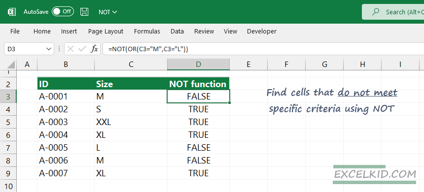
The formula in D3 is the following:
=NOT(OR(C3="M",C3="L"))We use text values in the test, so do not forget to use double quotes.
Explanation: The formula uses the following conditions: “the size is NOT “L” AND “M”. The formula will test all records in the range and returns TRUE if the size in column B is equal to “L” or “M”. So it is an OR relationship between the two conditions. If the t-shirt size is not “L” or “M” the formula will return FALSE.
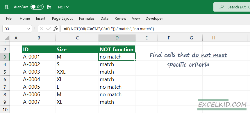
If you do not want to return booleans as output, make the formula easy to read using the IF function. Use a descriptive output for TRUE and FALSE results.
Formula:
=IF(NOT(OR(C3="M",C3="L")),"match","no match")Explanation: The IF function helps us create a descriptive name as an output. If the logical test is TRUE (we find the t-shirts where the size is not “M” or “L”), write “match”. Else, use the “no-match” string.
Example #2: Count non-blank cells in a range
If you want to count blank cells in a range, you can use the COUNTA function. In case of a cell status check, use the ISBLANK function. What if we want to highlight cells that are NOT blank?
Combine NOT and ISBLANK!
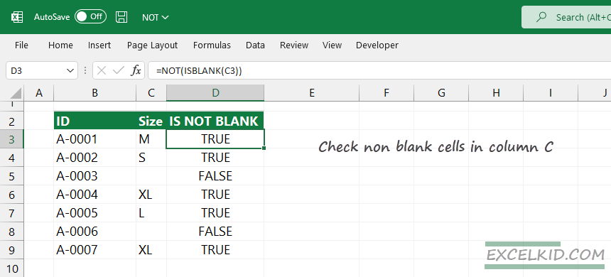
For the sake of simplicity, we use the same table:
=NOT(ISBLANK(C3))In this case, you can add the IF function if you want to display “blank” or “non-blank” outputs instead of TRUE or FALSE.
Additional resources: