The Excel GROUPBY function allows you to group, aggregate, sort, and filter data based on the specified fields.
GROUPBY is rolling out to users enrolled in the Windows and Mac Excel beta channels. You may shift to the Beta channel; if functionality is not available, it shall appear soon.
Table of contents:
- What is GROUPBY in Excel?
- How to use the GROUPBY function to aggregate data?
- GROUPBY Function Syntax and Arguments
- GROUPBY Function Examples
What is GROUPBY?
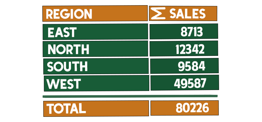
GROUPBY is a new dynamic array function in Microsoft Excel. The function uses three required and four optional arguments. GROUPBY allows you to create a summary of your data via a single formula. It supports grouping along one axis and aggregating the associated values. GROUPBY is lightweight, automatically updated, and can depend on the result of other calculations. Combine the function with other functions to create a percentage breakdown in seconds. For example, if you have a table of sales data, you can create a summary of sales by year.
How to use the GROUPBY function to aggregate data?
The function uses 3 required (and 4 optional) arguments.
Syntax:
=GROUPBY(row_fields, values, function, field_headers, total_depth, sort_order, filter_array)
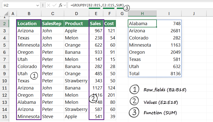
To do a simple GROUPBY in Excel, you need 3 arguments:
- What to group by
- The values to aggregate
- The function you’d like to use for the aggregation
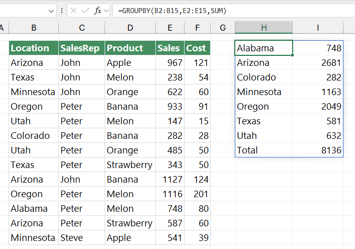
In the first example, we want to show how easy to create a Sales report by Location.
Formula:
=GROUPBY(B2:B15,E2:E15,SUM)
Select the column you want to group. Next, choose the column that contains values, in this case, Sales. Finally, choose a built-in function you want to use for the aggregation, in this case, sum.
Okay, it was a simple example.
GROUPBY Function Syntax and Arguments
In this chapter, we’ll explain all required and optional arguments.
Row fields
A column-oriented array or range containing the values used to group rows and generate row headers. The array or range may contain multiple columns. If so, the output will have multiple row group levels.
Values
Values is a column-oriented array or range of data to aggregate. The array or range may contain multiple columns. If so, the output will have multiple aggregations.
Function
The function argument is an explicit or eta-reduced lambda (SUM, PERCENTOF, AVERAGE, COUNT, etc.) used to aggregate values. A vector of lambdas can be provided. If so, the output will have multiple aggregations. The orientation of the vector will determine whether they are laid out row- or column-wise.
Field headers
A number specifies whether the row_fields and values have headers and whether field headers should be returned in the results. The possible values are:
- “0“: No; the data does not have headers and field headers should not be shown in the result.
- “1“: Yes, and don’t show; the field data has headers, but they should not be shown in the result.
- “2“: No, but generate; the field data does not have headers, but field headers should be generated and shown in the result.
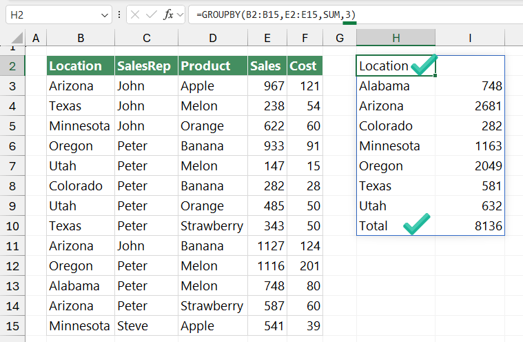
- “3“: Yes and show; the data has headers and field headers should be generated and shown in the result.
Here is an example of how to show headers and totals using “3” as a 4th argument.
Good to know: Automatic assumes the data contains headers based on the values argument. If the 1st value is text and the 2nd value is a number, then the data is assumed to have headers. Field headers are shown if there are multiple row or column group levels.
Total depth
Determines whether the row headers should contain totals.
The possible values are:
- Automatic without using the argument: Grand totals and, where possible, subtotals.
- “0“: No totals; do not show Totals
- “1“: Grand Totals; Show Grand Totals only
- “2“: Grand and Subtotals
- “-1“: Gran Totals at the top
- “-2“: Grand Totals and Subtotals at Top
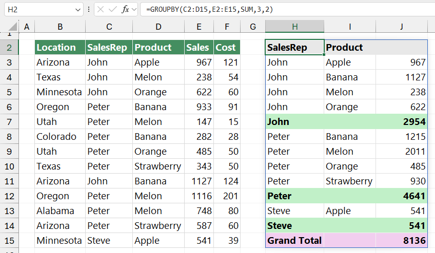
We want to show the Grand Totals and the Subtotals in the example. To do that, append the table and add a new category. We use the SalesRep and Product columns to demonstrate how the Totals work.
The formula looks like this:
=GROUPBY(C2:D15,E2:E15,SUM,3,2)
Sort Order
The sort_order argument is a number indicating how rows should be sorted. Numbers correspond with columns in row_fields followed by the columns in values. Using positive numbers, you can sort the data by ascending order. The rows are sorted in descending/reverse order if the value is negative.
A vector of numbers can be provided when sorting based on only row fields.
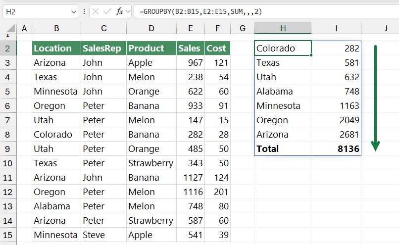
Okay, back to the previous example! We want to apply an ascending order for column 2!
Formula:
=GROUPBY(B2:B15,E2:E15,SUM,,,2)
Filter array
The last argument is the filter array. The filter_array is a column-oriented 1D array of Booleans that indicates whether the corresponding row of data should be considered. You can filter the result using logical expressions to decide which record to exclude.
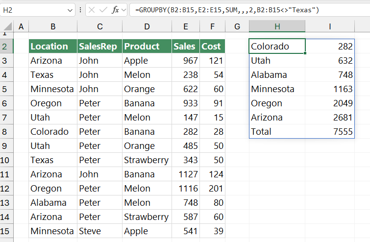
If you want to exclude Texas in the Location column, simply use this expression.
=GROUPBY(B2:B15,E2:E15,SUM,,,2,B2:B15<>”Texas”)
GROUPBY Function Examples
In this section, we will demonstrate some useful GROUPBY function examples.
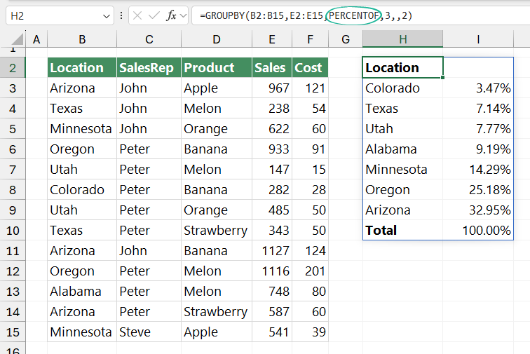
Combine GROUPBY with the PERCENTOF function
As mentioned above, GROUPBY can use 16 different functions as an argument, so it does not need to use LAMBDA to perform various calculations. Try to use the PERCENTOF function to create a breakdown.
Locate the third argument, replace the sum function with the PERCENTOF function, and press enter. The result looks great; now you have a percentage breakdown by location. Finally, as a result of the formula, you achieved this dynamic array without using any Pivot Tables. So, it is a stunning way to save time and keep your tables up to date.
You can use other built-in functions like AVERAGE, MEDIAN, MIN, MAX, COUNT, and CONCAT. The method is the same as above; replace the “function” argument.